背景
在很多情况下缺失真实场景的数据来训练模型,因此学术界提出非常多的自监督、半监督、无监督学习模型来缓解训练数据不足的情况。但整体而言,缺少监督数据训练的模型性能往往会弱于监督模型,目前落地的大部分 AI-DNN 都是建立在海量的训练数据基础上。
为了提高模型的学习能力,可以利用 Data Augmentation 技术来扩大训练数据集,这一方法在 CV 领域尤为成熟。虽然人工生成的数据与真实场景存在一定的 gap,但对模型的性能仍会有一定提升。
对于时序领域,本文学习下经典的时间序列数据生成模型 「TimeGAN」,并基于 ydata-synthetic 库验证其生成的时间序列效果。
TimeGAN
TimeGAN (Time-series Generative Adversarial Network) 是一种时间序列数据生成模型,由加州大学 Jinsung Yoon 等人在 NeurIPS 2019 中提出。[^1] 主要想法是将无监督 GAN 方法的多功能性与对有监督的自回归模型提供的条件概率原理结合,来生成保留时间动态的时间序列。详细理论不再赘述,主要想测试下其性能和生成序列的效果。
此处附上论文下载链接及源码地址,感兴趣可以深入学习。
论文链接:https://openreview.net/forum?id=rJeZq4reLS
源码链接:https://github.com/jsyoon0823/TimeGAN
Python 实践
本文中直接基于 ydata-synthetic 库中 TimeGAN 实验进行测试,不想再解决原始库中的版本依赖问题。
ydata-synthetic 中包含一系列 GAN 模型来合成数据, 例如 TimeGAN、CGAN、WGAN 等等,也可以生成欺诈数据等表格式数据。此处用到的是 TimeGAN 来生成时间序列数据,同时包含一个 Yahoo 股票序列数据生成示例。
原始数据下载:https://finance.yahoo.com/quote/GOOG/history?p=GOOG
处理数据下载:Github/dreamhomes stock_data.csv
源码参考:Google Colab TimeGAN
代码主要包含以下 5 个流程:
「加载数据并选择参数」
from os import path

import pandas as pd
import numpy as np
import matplotlib.pyplot as plt
import matplotlib.gridspec as gridspec

from ydata_synthetic.synthesizers import ModelParameters
from ydata_synthetic.preprocessing.timeseries import processed_stock
from ydata_synthetic.synthesizers.timeseries import TimeGAN

seq_len=24
n_seq = 6
hidden_dim=24
gamma=1

noise_dim = 32
dim = 128
batch_size = 128

log_step = 100
learning_rate = 5e-4

stock_data = processed_stock(path='../../data/stock_data.csv', seq_len=seq_len)
print(len(stock_data),stock_data[0].shape)
「模型初始化训练」
📢 注意:模型训练速度慢,可以减少 epochs 数量,例如 train_steps=10000
gan_args = ModelParameters(batch_size=batch_size,
                           lr=learning_rate,
                           noise_dim=noise_dim,
                           layers_dim=dim)
synth = TimeGAN(model_parameters=gan_args, hidden_dim=24, seq_len=seq_len, n_seq=n_seq, gamma=1)
synth.train(stock_data, train_steps=50000)
synth.save('synthesizer_stock.pkl')
「生成序列数据」
synth_data = synth.sample(len(stock_data))
print(synth_data.shape)
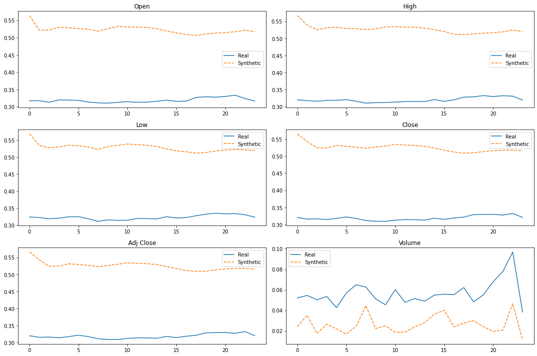
「序列数据可视化」
#Reshaping the data
cols = ['Open','High','Low','Close','Adj Close','Volume']

#Plotting some generated samples. Both Synthetic and Original data are still standartized with values between [0,1]
fig, axes = plt.subplots(nrows=3, ncols=2, figsize=(15, 10))
axes=axes.flatten()

time = list(range(1,25))
obs = np.random.randint(len(stock_data))

for j, col in enumerate(cols):
    df = pd.DataFrame({'Real': stock_data[obs][:, j],
                   'Synthetic': synth_data[obs][:, j]})
    df.plot(ax=axes[j],
            title = col,
            secondary_y='Synthetic data', style=['-', '--'])
fig.tight_layout()
「评价数据分布(PCA+t-SNE)」
from sklearn.decomposition import PCA
from sklearn.manifold import TSNE

sample_size = 250
idx = np.random.permutation(len(stock_data))[:sample_size]

real_sample = np.asarray(stock_data)[idx]
synthetic_sample = np.asarray(synth_data)[idx]

#for the purpose of comparision we need the data to be 2-Dimensional. For that reason we are going to use only two componentes for both the PCA and TSNE.
synth_data_reduced = real_sample.reshape(-1, seq_len)
stock_data_reduced = np.asarray(synthetic_sample).reshape(-1,seq_len)

n_components = 2
pca = PCA(n_components=n_components)
tsne = TSNE(n_components=n_components, n_iter=300)

#The fit of the methods must be done only using the real sequential data
pca.fit(stock_data_reduced)

pca_real = pd.DataFrame(pca.transform(stock_data_reduced))
pca_synth = pd.DataFrame(pca.transform(synth_data_reduced))

data_reduced = np.concatenate((stock_data_reduced, synth_data_reduced), axis=0)
tsne_results = pd.DataFrame(tsne.fit_transform(data_reduced))

fig = plt.figure(constrained_layout=True, figsize=(20,10))
spec = gridspec.GridSpec(ncols=2, nrows=1, figure=fig)

#TSNE scatter plot
ax = fig.add_subplot(spec[0,0])
ax.set_title('PCA results',
             fontsize=20,
             color='red',
             pad=10)

#PCA scatter plot
plt.scatter(pca_real.iloc[:, 0].values, pca_real.iloc[:,1].values,
            c='black', alpha=0.2, label='Original')
plt.scatter(pca_synth.iloc[:,0], pca_synth.iloc[:,1],
            c='red', alpha=0.2, label='Synthetic')
ax.legend()

ax2 = fig.add_subplot(spec[0,1])
ax2.set_title('TSNE results',
              fontsize=20,
              color='red',
              pad=10)

plt.scatter(tsne_results.iloc[:sample_size, 0].values, tsne_results.iloc[:sample_size,1].values,
            c='black', alpha=0.2, label='Original')
plt.scatter(tsne_results.iloc[sample_size:,0], tsne_results.iloc[sample_size:,1],
            c='red', alpha=0.2, label='Synthetic')

ax2.legend()

fig.suptitle('Validating synthetic vs real data diversity and distributions',
             fontsize=16,
             color='grey')
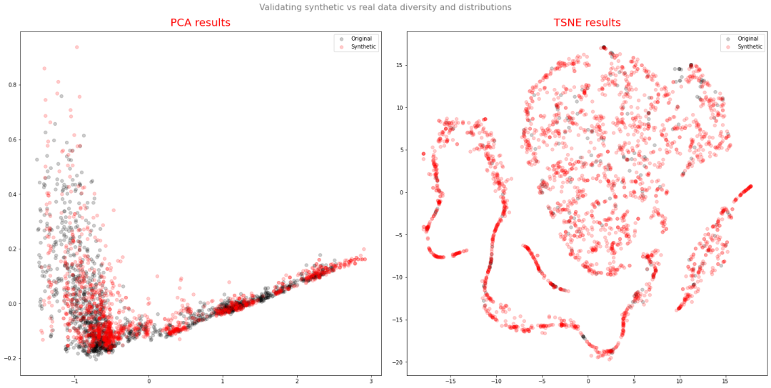
整体而言 TimeGAN 生成的序列符合真实序列的趋势,而且时间序列分布大体上与真实序列相同。因此,在缺少真实时间序列数据的情况下可以使用来训练模型!
[^1]: Yoon, Jinsung, Daniel Jarrett, and Mihaela Van der Schaar. "Time-series generative adversarial networks." (2019).

● KDD 2021丨RANSynCoder:异步多变量时间序列异常检测与定位模型
● KDD 2020 | MTGNN: 基于图神经网络的多变量时间序列预测模型

 「阅读原文」留言