数据集中的类不平衡问题与过采样方法对比

背景

数据类不平衡问题（Class-imbalance）是指在训练分类模型时所使用的训练集的标签类别分布不均匀。例如正类样本995个，负类样本仅5个（少数类），这样的数据集中就存在类不平衡问题。

对于不平衡类的研究通常认为不平衡意味着少数类只占少于10%到20%。

“

对于数据集中类别不平衡的问题是否需要特殊处理，需要取决于训练出来的模型在验证集中的效果，如果效果较好说明没有必要进行处理。

类不平衡导致的问题可能导致模型出现问题，模型训练过程中某类的样本数量太少说明在训练过程中提供的“特征信息”少，模型对少数类的判定效果差。可能由于验证集准确率较高而终止优化那么会导致模型不知如何去判别出少数类。

解决方案

对于数据不平衡问题，当前有不同的方法来缓解：

• 取决于数据，不处理时可能效果也不差。
• 数据层面上通过某种方法是数据更加平衡：
• 对于少数类进行过采样；
• 对于多数类进行欠采样；
• 合成新的少数类样本；
• 舍弃所有少数类，使用异常检测框架。
• 算法层面上调整模型：
• 调整类权重；
• 调整决策阈值；
• 使用已有的算法对少数类更加敏感；
• 构造一个在不平衡数据上表现效果好的全新算法。

注意： 对于不平衡类分类器不要使用准确率（Accuracy）作为评价指标，准确率通常以0.5作为概率阈值来判定所属类别，在不平衡数据集中通常会出错。一般使用ROC、AUC曲线，F1分数。

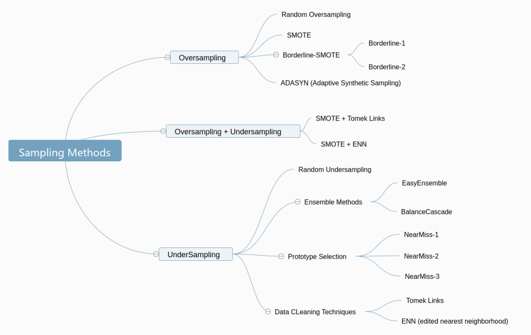
列出一张相关采样方法导图：

本文主要学习下常用的 SMOTE 采样方法。

参考：不同过采样方法之间的量化比较^[1]

SMOTE 过采样方法

SMOTE 采样

SMOTE 基于“插值”的方法为少数类合成新的样本。

设少数类的样本数为 ，那么SMOTE将为少数类合成 个新样本，其中 为正整数。

假设少数类中的一个样本 ，特征向量为 ,：

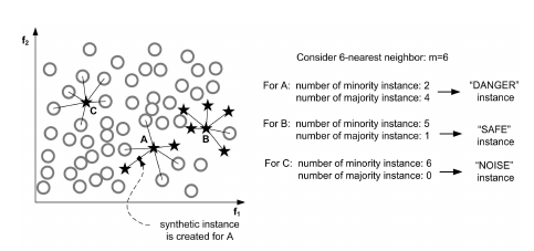
1. 首先从该少数类 个样本中选择 的 个近邻样本（采用欧式距离），记为 ;

2. 然后从 个进行的样本中随机选择一个样本 ，在生成0到1间的随机数 ,可以合成一个新的样本 :

3. 将步骤 2 重负执行 次，从而可以合成 个新样本：。

因此，对所有的 个少数类样本执行上述操作即可合成 个新样本。

SMOTE会随机选取少数类样本用以合成新样本，而不考虑周边样本的情况，这样容易带来两个问题：

1. 如果选取的少数类样本周围也都是少数类样本，则新合成的样本不会提供太多有用信息。这就像支持向量机中远离margin的点对决策边界影响不大。
2. 如果选取的少数类样本周围都是多数类样本，这类的样本可能是噪音，则新合成的样本会与周围的多数类样本产生大部分重叠，致使分类困难。

总体来说我们希望新合成的少数类样本能处于两个类别的边界附近，这样往往能提供足够的信息用以分类。

Borderline SMOTE 采样

对于SMOTE方法，Borderline-SMOTE中增加少数类中样本的选择过程。根据所有k-NN样本将少数类样本分为三类：

• “noise” instance：所有的 kNN 样本都属于多数类；
• “danger” instance：超过一半的 kNN 样本属于多数类；
• “safe” instance：超过一半的 kNN 样本属于少数类；

Borderline SMOTE
算法只会从处于danger状态的样本中随机选择，然后用SMOTE算法产生新的样本。处于danger状态的样本代表靠近边界附近的少数类样本，而处于边界附近的样本往往更容易被误分类。因而 Borderline SMOTE
只对那些靠近边界的少数类样本进行人工合成样本，而 SMOTE
则对所有少数类样本一视同仁。

Border-line SMOTE分为两种: Borderline-1 SMOTE和Borderline-2 SMOTE。Borderline-1 SMOTE在合成样本时式中的 是一个少数类样本，而Borderline-2 SMOTE中的 则是k近邻中的任意一个样本。

SVM SMOTE 采样

使用一个SVM分类器寻找支持向量，然后在支持向量的基础上合成新的样本。类似Broderline Smote,SVM smote也会根据K近邻的属性决定样本的类型（safe,danger,noice）,然后使用danger的样本训练SVM。

Kmeans SMOTE 采样

在合成样本之前先对样本进行聚类，然后根据簇密度的大小分别对不同簇的负样本进行合成。在聚类步骤中，使用k均值聚类为k个组。过滤选择用于过采样的簇，保留具有高比例的少数类样本的簇。然后，它分配合成样本的数量，将更多样本分配给少数样本稀疏分布的群集。最后，过采样步骤，在每个选定的簇中应用SMOTE以实现少数和多数实例的目标比率。

SMOTE-NC 采样

以上的Smote方法都不能处理分类变量，SMOTE-NC由于分类变量无法计算插值，SMOTE-NC会在合成新样本的时候参考新样本最近邻的该特征，然后区其中出现次数最多的值。

Python 实现

SMOTE 的一个主流实现是来自于sklearn的contrib项目imbalanced_learn
，使用imbalanced_learn的smote符合sklearn的API规范。

参考：imbalanced-learn/SMOTE^[2]

from sklearn.datasets import make_classification
from imblearn.over_sampling import SMOTE
from collections import Counter


X, y = make_classification(n_classes=2, class_sep=2, weights=[0.1, 0.9], n_informative=1, n_redundant=1, flip_y=0,
                           n_features=2, n_clusters_per_class=1, n_samples=1000, random_state=10)
# Counter(y)
# Counter({1: 900, 0: 100})
sm = SMOTE(random_state=42)
X_res, y_res = sm.fit_resample(X, y)
# Counter(y_res)
# Counter({1: 900, 0: 900})

不同过采样方法的比较

from collections import Counter

import matplotlib.pyplot as plt
import numpy as np

from sklearn.datasets import make_classification
from sklearn.svm import LinearSVC

from imblearn.pipeline import make_pipeline
from imblearn.over_sampling import ADASYN
from imblearn.over_sampling import (SMOTE, BorderlineSMOTE, SVMSMOTE, SMOTENC, KMeansSMOTE)
from imblearn.over_sampling import RandomOverSampler
from imblearn.base import BaseSampler

# 生成不平衡数据集
def create_dataset(n_samples=1000, weights=(0.01, 0.01, 0.98), n_classes=3,
                   class_sep=0.8, n_clusters=1):
    return make_classification(n_samples=n_samples, n_features=2,
                               n_informative=2, n_redundant=0, n_repeated=0,
                               n_classes=n_classes,
                               n_clusters_per_class=n_clusters,
                               weights=list(weights),
                               class_sep=class_sep, random_state=0)


# 图展示过采样结果
def plot_resampling(X, y, sampling, ax):
    X_res, y_res = sampling.fit_resample(X, y)
    ax.scatter(X_res[:, 0], X_res[:, 1], c=y_res, alpha=0.8, edgecolor='k')
    # make nice plotting
    ax.spines['top'].set_visible(False)
    ax.spines['right'].set_visible(False)
    ax.get_xaxis().tick_bottom()
    ax.get_yaxis().tick_left()
    ax.spines['left'].set_position(('outward', 10))
    ax.spines['bottom'].set_position(('outward', 10))
    return Counter(y_res)

## 判别函数结果
def plot_decision_function(X, y, clf, ax):
    plot_step = 0.02
    x_min, x_max = X[:, 0].min() - 1, X[:, 0].max() + 1
    y_min, y_max = X[:, 1].min() - 1, X[:, 1].max() + 1
    xx, yy = np.meshgrid(np.arange(x_min, x_max, plot_step),
                         np.arange(y_min, y_max, plot_step))

    Z = clf.predict(np.c_[xx.ravel(), yy.ravel()])
    Z = Z.reshape(xx.shape)
    ax.contourf(xx, yy, Z, alpha=0.4)
    ax.scatter(X[:, 0], X[:, 1], alpha=0.8, c=y, edgecolor='k')

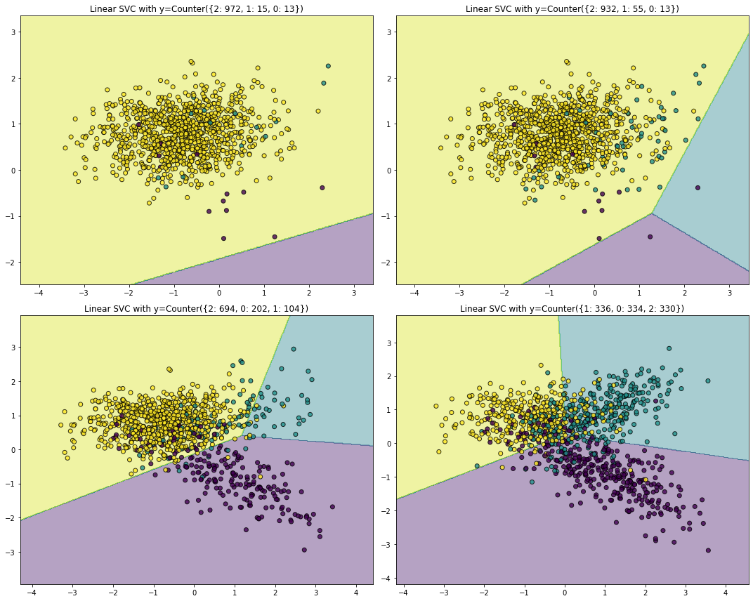
X, y = create_dataset()
Counter(y)

Counter({2: 972, 1: 15, 0: 13})

# 验证数据不同平衡率对模型的影响，如线性SVM
fig, ((ax1, ax2), (ax3, ax4)) = plt.subplots(2, 2, figsize=(15, 12))

ax_arr = (ax1, ax2, ax3, ax4)
weights_arr = ((0.01, 0.01, 0.98), (0.01, 0.05, 0.94),
               (0.2, 0.1, 0.7), (0.33, 0.33, 0.33))
for ax, weights in zip(ax_arr, weights_arr):
    X, y = create_dataset(n_samples=1000, weights=weights)
    clf = LinearSVC().fit(X, y)
    plot_decision_function(X, y, clf, ax)
    ax.set_title('Linear SVC with y={}'.format(Counter(y)))
fig.tight_layout()

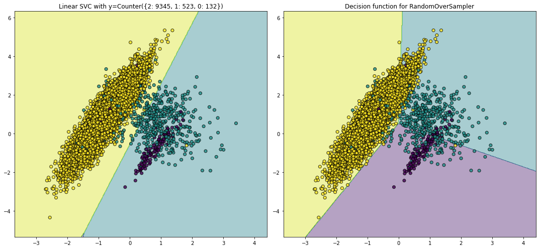
# 采用随机采样来平衡数据集：
fig, (ax1, ax2) = plt.subplots(1, 2, figsize=(15, 7))
X, y = create_dataset(n_samples=10000, weights=(0.01, 0.05, 0.94))
clf = LinearSVC().fit(X, y)
plot_decision_function(X, y, clf, ax1)
ax1.set_title('Linear SVC with y={}'.format(Counter(y)))
pipe = make_pipeline(RandomOverSampler(random_state=0), LinearSVC())
pipe.fit(X, y)
plot_decision_function(X, y, pipe, ax2)
ax2.set_title('Decision function for RandomOverSampler')
fig.tight_layout()

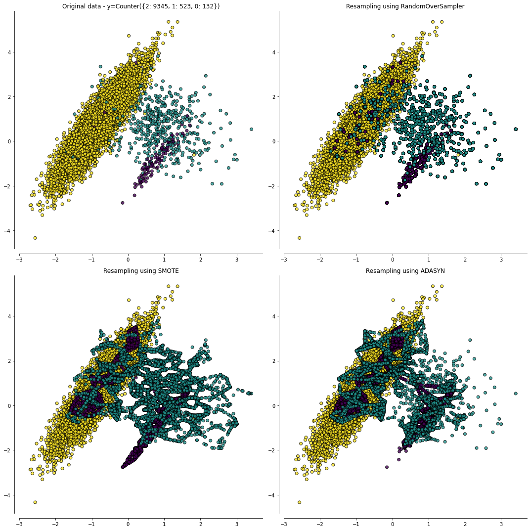
## 其它高级的过采样算法：ADASYN和SMOTE
class FakeSampler(BaseSampler):

    _sampling_type = 'bypass'

    def _fit_resample(self, X, y):
        return X, y


fig, ((ax1, ax2), (ax3, ax4)) = plt.subplots(2, 2, figsize=(15, 15))
X, y = create_dataset(n_samples=10000, weights=(0.01, 0.05, 0.94))
sampler = FakeSampler()
clf = make_pipeline(sampler, LinearSVC())
plot_resampling(X, y, sampler, ax1)
ax1.set_title('Original data - y={}'.format(Counter(y)))

ax_arr = (ax2, ax3, ax4)
for ax, sampler in zip(ax_arr, (RandomOverSampler(random_state=0),
                                SMOTE(random_state=0),
                                ADASYN(random_state=0))):
    clf = make_pipeline(sampler, LinearSVC())
    clf.fit(X, y)
    plot_resampling(X, y, sampler, ax)
    ax.set_title('Resampling using {}'.format(sampler.__class__.__name__))
fig.tight_layout()

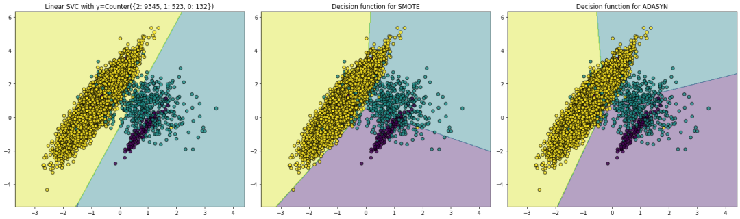
fig, (ax1, ax2, ax3) = plt.subplots(1, 3, figsize=(20, 6))
X, y = create_dataset(n_samples=10000, weights=(0.01, 0.05, 0.94))

clf = LinearSVC().fit(X, y)
plot_decision_function(X, y, clf, ax1)
ax1.set_title('Linear SVC with y={}'.format(Counter(y)))
sampler = SMOTE()
clf = make_pipeline(sampler, LinearSVC())
clf.fit(X, y)
plot_decision_function(X, y, clf, ax2)
ax2.set_title('Decision function for {}'.format(sampler.__class__.__name__))
sampler = ADASYN()
clf = make_pipeline(sampler, LinearSVC())
clf.fit(X, y)
plot_decision_function(X, y, clf, ax3)
ax3.set_title('Decision function for {}'.format(sampler.__class__.__name__))
fig.tight_layout()

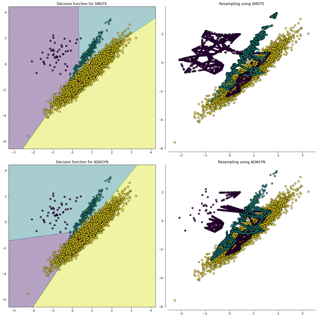
# 不同过采样方法对分类器的影响
fig, ((ax1, ax2), (ax3, ax4)) = plt.subplots(2, 2, figsize=(15, 15))
X, y = create_dataset(n_samples=5000, weights=(0.01, 0.05, 0.94),
                      class_sep=0.8)

ax_arr = ((ax1, ax2), (ax3, ax4))
for ax, sampler in zip(ax_arr, (SMOTE(random_state=0),
                                ADASYN(random_state=0))):
    clf = make_pipeline(sampler, LinearSVC())
    clf.fit(X, y)
    plot_decision_function(X, y, clf, ax[0])
    ax[0].set_title('Decision function for {}'.format(
        sampler.__class__.__name__))
    plot_resampling(X, y, sampler, ax[1])
    ax[1].set_title('Resampling using {}'.format(
        sampler.__class__.__name__))
fig.tight_layout()

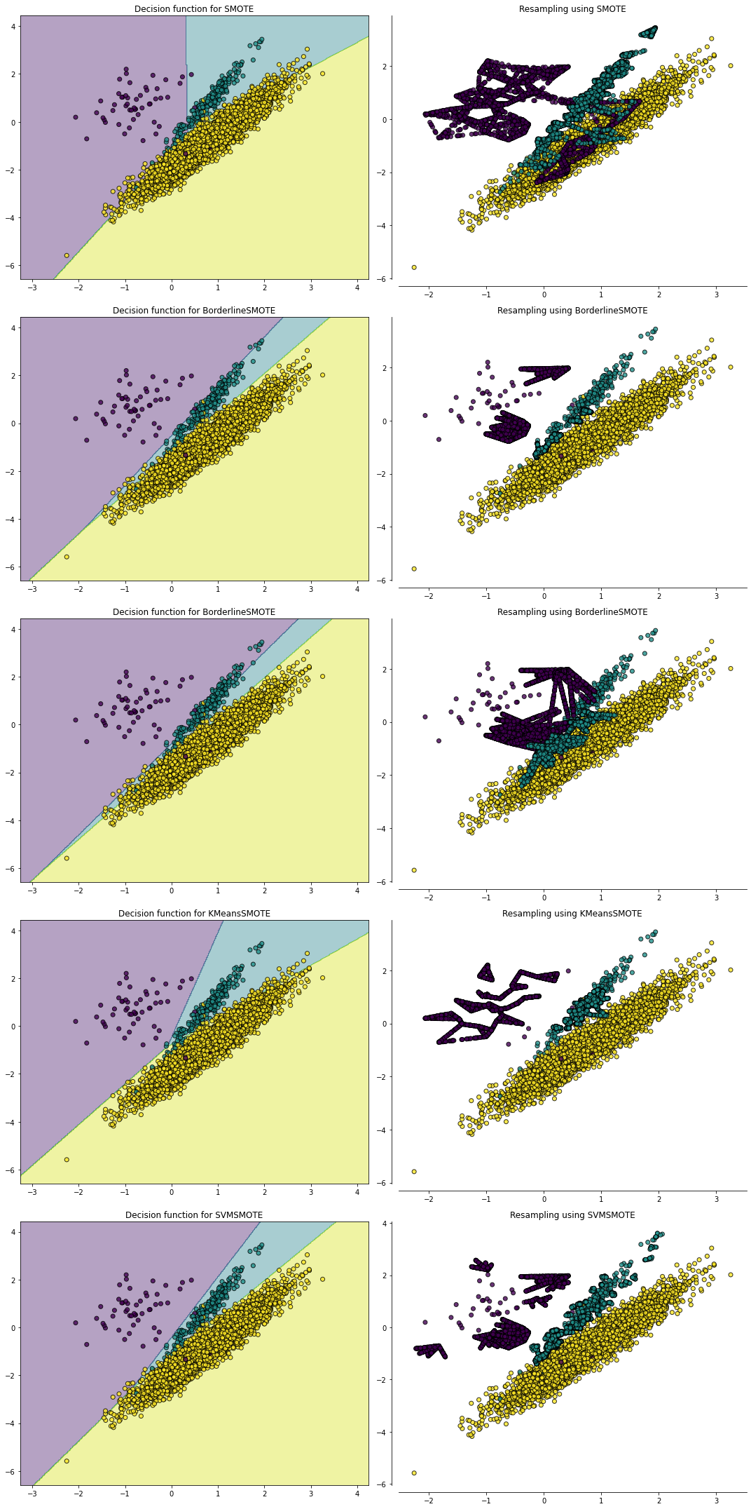
# 考虑不同SMOTE变种算法对分类器的影响
fig, ((ax1, ax2), (ax3, ax4),
      (ax5, ax6), (ax7, ax8),
      (ax9, ax10)) = plt.subplots(5, 2, figsize=(15, 30))
X, y = create_dataset(n_samples=5000, weights=(0.01, 0.05, 0.94),
                      class_sep=0.8)


ax_arr = ((ax1, ax2), (ax3, ax4), (ax5, ax6), (ax7, ax8), (ax9, ax10))
for ax, sampler in zip(ax_arr,
                       (SMOTE(random_state=0),
                        BorderlineSMOTE(random_state=0, kind='borderline-1'),
                        BorderlineSMOTE(random_state=0, kind='borderline-2'),
                        KMeansSMOTE(random_state=0),
                        SVMSMOTE(random_state=0))):
    clf = make_pipeline(sampler, LinearSVC())
    clf.fit(X, y)
    plot_decision_function(X, y, clf, ax[0])
    ax[0].set_title('Decision function for {}'.format(
        sampler.__class__.__name__))
    plot_resampling(X, y, sampler, ax[1])
    ax[1].set_title('Resampling using {}'.format(sampler.__class__.__name__))
fig.tight_layout()

# 使用SMOTE-NC来处理连续变量与离散变量特征
rng = np.random.RandomState(42)
n_samples = 50
X = np.empty((n_samples, 3), dtype=object)
X[:, 0] = rng.choice(['A', 'B', 'C'], size=n_samples).astype(object)
X[:, 1] = rng.randn(n_samples)
X[:, 2] = rng.randint(3, size=n_samples)
y = np.array([0] * 20 + [1] * 30)

print('The original imbalanced dataset')
print(sorted(Counter(y).items()))
print('The first and last columns are containing categorical features:')
print(X[:5])

smote_nc = SMOTENC(categorical_features=[0, 2], random_state=0)
X_resampled, y_resampled = smote_nc.fit_resample(X, y)
print('Dataset after resampling:')
print(sorted(Counter(y_resampled).items()))
print('SMOTE-NC will generate categories for the categorical features:')
print(X_resampled[-5:])

The original imbalanced dataset
[(0, 20), (1, 30)]
The first and last columns are containing categorical features:
[['C' -0.14021849735700803 2]
 ['A' -0.033193400066544886 2]
 ['C' -0.7490765234433554 1]
 ['C' -0.7783820070908942 2]
 ['A' 0.948842857719016 2]]
Dataset after resampling:
[(0, 30), (1, 30)]
SMOTE-NC will generate categories for the categorical features:
[['A' 0.5246469549655818 2]
 ['B' -0.3657680728116921 2]
 ['B' 0.9344237230779993 2]
 ['B' 0.3710891618824609 2]
 ['B' 0.3327240726719727 2]]

参考资料