前言
在之前的文章任意网页正文内容主题词提取中,我们采用了一个tf-idf来获取本文的关键词(主题)。由于tf-idf算法仅仅是一个统计模型,简单快速,适合作为baseline。它最大的问题在于单单考虑了词频,而没有考虑语义,并且我们取topK的词,这个K值如何选取,也是一个问题。本文介绍一种真正的主题模型,也是最早出现的主题模型LSA(Latent Semantic Analysis):潜在语义分析,它主要是利用SVD降维的方式,将词与本文映射到一个新的空间,而这个空间正是以主题作为维度。它的原理非常漂亮,一次奇异值分解就可以得到主题模型,同时也解决了词义的问题。本文继续发挥hands-on的传统,以一个实例来说明LSA的用法。在生产环境中,一般会使用gensim等框架来快速进行开发,本文从scipy和numpy入手,可以更清楚的了解其中的原理。
数据预处理
为了演示方便,我们直接采用了scikit-learn中的Newsgroups数据集。这是用于文本分类、文本挖据和信息检索研究的国际标准数据集之一。数据集收集了大约20,000左右的新闻组文档,均匀分为20个不同主题的新闻组集合。我们截取了其中4个主题的数据,并采用scikit-learn中的API来装载。
from sklearn.datasets import fetch_20newsgroupscategories = ['alt.atheism', 'talk.religion.misc', 'comp.graphics', 'sci.space']remove = ('headers', 'footers', 'quotes')newsgroups_train = fetch_20newsgroups(subset='train', categories=categories, remove=remove)newsgroups_test = fetch_20newsgroups(subset='test', categories=categories, remove=remove)
数据下载好后,我们看看里面的文本长啥样
newsgroups_train.data[:2]'''["Hi,\n\nI've noticed that if you only save a model (with all your mapping planes\npositioned carefully) to a .3DS file that when you reload it after restarting\n3DS, they are given a default position and orientation. But if you save\nto a .PRJ file their positions/orientation are preserved. Does anyone\nknow why this information is not stored in the .3DS file? Nothing is\nexplicitly said in the manual about saving texture rules in the .PRJ file. \nI'd like to be able to read the texture rule information, does anyone have \nthe format for the .PRJ file?\n\nIs the .CEL file format available from somewhere?\n\nRych",'\n\nSeems to be, barring evidence to the contrary, that Koresh was simply\nanother deranged fanatic who thought it neccessary to take a whole bunch of\nfolks with him, children and all, to satisfy his delusional mania. Jim\nJones, circa 1993.\n\n\nNope - fruitcakes like Koresh have been demonstrating such evil corruption\nfor centuries.']'''
拿到文本后,第一件事当然是tokenizer,然后采用bag-of-words词袋模型将其向量化。这里使用scikit-learn中的CountVectorizer
,以词频计数来作为向量值,当然更精细化可以采用TfidfVectorizer
。
import numpy as npfrom sklearn.feature_extraction.text import CountVectorizervectorizer = CountVectorizer(stop_words='english')vectors = vectorizer.fit_transform(newsgroups_train.data).todense()vocab = np.array(vectorizer.get_feature_names())
可以看看向量化后的矩阵
vectors.shape'''(2034, 26576)'''
这里表示共有2034篇文档,词的vocab_size为26576,将所有文档转成了26576维的向量,每个向量的值为该维表示词的词频。
SVD分解
向量化完成后,我们就可以开始奇异值分解了。
import scipyU, s, Vh = scipy.linalg.svd(vectors, full_matrices=False)
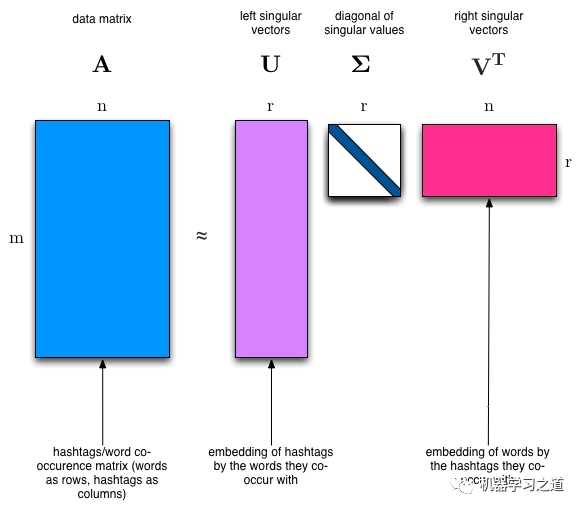
根据上图,我们可以看到分解出来的矩阵:
•U: (2034, 2034) 表示2034个样本,对应2034个topic•s: (2034, ) 表示2034个奇异值,即topic的重要性分数•Vh: (2034, 26576) 表示2034个topic,对应26576个vocab,注意这个Vh是公式中的VT,即转置后的V SVD奇异值分解,具有以下性质:•奇异值分解为精确分解,即分解后的矩阵可以完全还原原矩阵,信息不丢失•U和Vh是正交矩阵 我们可以在numpy中验证一下:
# 注意将s从一维向量转换成对角矩阵(diagonal matrix)np.allclose(U.dot(np.diag(s)).dot(Vh), vectors) # Truenp.allclose(U.T.dot(U), np.eye(U.shape[0])) # Truenp.allclose(Vh.dot(Vh.T), np.eye(Vh.shape[0])) # True
Topic解读
LSA的优雅之处,就是把之前的高维文档向量,降维到低维,且这个维度代表了文档的隐含语义,即这个文档的主题topic。svd分解出来的Vh矩阵,即是每个主题的矩阵,维度是每个单词,维度值可以看成是这个主题中每个单词的的重要性。那么,我们可以选取重要性最高的词,来解读某个隐含主题。
num_top_words = 8def show_topics(a):top_words = lambda t: [vocab[i] for i in np.argsort(t)[:-num_top_words-1:-1]]topic_words = ([top_words(t) for t in a])return [' '.join(t) for t in topic_words]show_topics(Vh[:10])'''['ditto critus propagandist surname galacticentric kindergarten surreal imaginative','jpeg gif file color quality image jfif format','graphics edu pub mail 128 3d ray ftp','jesus god matthew people atheists atheism does graphics','image data processing analysis software available tools display','god atheists atheism religious believe religion argument true','space nasa lunar mars probe moon missions probes','image probe surface lunar mars probes moon orbit','argument fallacy conclusion example true ad argumentum premises','space larson image theory universe physical nasa material']'''
可以看出,有些主题是关于图片格式的,有的是关于邮件协议的,有的是关于太空的。而svd分解出来的U矩阵,就是每个文档对应的主题矩阵,维度是每个主题,维度值也可以看成是每个主题的重要性。
Truncated SVD
在生产实践中,普通svd由于要exact decomposition,计算量会非常大,且最后的应用往往会只看前n个topic,因此Truncated SVD的优势在于,预先设置好n的值,可以在牺牲一定精度的条件下,大大减少计算量。这里提供两种常见的svd实现以作参考。 sklearn实现
from sklearn import decompositionu, s, v = decomposition.randomized_svd(vectors, 10)
Facebook实现
import fbpcau, s, v = fbpca.pca(vectors, 10)
总结
LSA作为最早出现的真正主题模型,非常优雅,同时也存在很多不足,比如它得到的不是一个概率模型,同时得到的向量中含有负值,难以直观解释。针对这些问题,后续就有NMF(非负矩阵分解),LDA(隐含狄利克雷分布)等模型出现。
最后
欢迎订阅我的微信公众号“机器学习之道”,第一时间免费收到文章更新。