


7.1 introduction
Chapter 2 showed the increase in precision that can come from using population data to stratify sampling.
第 2 章展示了使用总体数据对抽样进行分层可以提高精度。
Stratification is not always a desirable way to use these population data: there may be too many potential stratification variables, the best strata may be different for different analyses, or the need for cluster sampling may prevent stratification on individual-level variables.
分层并不总是使用这些总体数据的理想方式:可能有太多的潜在分层变量,不同分析的最佳分层可能不同,或者整群抽样的需要可能会阻止对个人水平变量进行分层。
Population data may also be available in a form that does not allow for stratification - random-digit dialing, for example, cannot easily stratify on any individual characteristics, because these characteristics are not known before dialing and so cannot be used to select the sample.
人口数据也可能以不允许分层的形式提供——例如,随机数字拨号不能轻易地对任何个人特征进行分层,因为这些特征在拨号之前是未知的,因此不能用于选择样本。
This chapter deals with techniques for using known population totals for a set of variables (uuxiZiury variables) to adjust the sampling weights and improve estimation for another set of variables.
本章介绍使用一组变量(uuxiZiury变量)的已知总体总数来调整抽样权重并改进对另一组变量的估计的技术。
All of these techniques have the same idea: adjustments are made to the sampling weights so that estimated population totals for the auxiliary variables match the known population totals, making the sample more representative of the population.
所有这些技术都有相同的想法:对抽样权重进行调整,以便辅助变量的估计总体总数与已知总体总数相匹配,从而使样本更能代表总体。
A second benefit is that the estimates are forced to be consistent with the population data, improving their credibility with people who may not understand the sampling process.
第二个好处是,估计被迫与人口数据一致,从而提高自己的信誉的人谁可能不明白的采样过程。
There are two quite different applications of these techniques.
这些技术有两种截然不同的应用。
One is to increase precision of estimation, the other is to reduce the bias from nonresponse, especially unit non-response, where a sampled individual refuses to participate or otherwise provides no information for analysis.
一是提高估计的精确度,二是减少无响应的偏差,尤其是单位无响应,在这种情况下,被抽样的个人拒绝参与或以其他方式不提供分析信息。
From the computational viewpoint the main difference between these applications is in the criteria for choosing auxiliary variables, which are discussed in section 7.6.
从计算的角度来看,这些应用程序之间的主要区别在于选择辅助变量的标准,这将在第 7.6 节中讨论。
The use for non-response is the more important of the two in large-scale surveys, but it has largely been completed by the time the data arrive at the typical user.
在大规模调查中,不答复的使用是两者中更重要的一个,但在数据到达典型用户时已经基本完成。
Calibration to improve precision will be important in the two-phase epidemiologic designs discussed in Chapter 8.
在第 8 章讨论的两阶段流行病学设计中,校准以提高精确度非常重要。
Item non-response, where some variables but not others were observed for an individual is addressed in Chapter 9.
第 9 章讨论了项目不答复,即针对个人观察到了一些变量而不是其他变量。
7.2 post-stratification
The simplest technique for adjusting sampling weights is post-stratification.
调整采样权重的最简单技术是后分层。
Suppose we have a division of the population into groups.
假设我们将人口分成几组。
One possible design would be a stratified random sample using these groups as strata, sampling nk individuals from population stratum k containing Nk individuals.
一种可能的设计是使用这些组作为层的分层随机样本,从包含Nk 个个体的人口层 k 中抽样nk个个体。
The sampling weights are l/ni = Nk/?lk and the Horvitz-Thompson estimator f i k of the population group size is exactly correct and its standard error is zero.
抽样权重为l/ni = Nk/?lk ,总体群体规模的 Horvitz-Thompson 估计量fik完全正确,其标准误差为零。
Estimation of other population totals is improved by removing the variability between groups: the contribution of each group to a population total is fixed by design, rather than random.
通过消除组之间的可变性来改进对其他总体总数的估计:每个组对总体总数的贡献是由设计固定的,而不是随机的。
If Nk were known, but the sampling was not stratified, the estimated population group sizes would not be exactly correct.
如果Nk已知,但抽样未分层,则估计的人口组大小将不完全正确。
Post-stratification adjusts the sampling weights so that the estimated population group sizes are correct, as they would be in stratified sampling.
后分层调整采样的权重,从而使估计人口组大小是正确的,因为他们将在分层抽样。
The sampling weights l/ni are replaced by weights g i n i where gi = Nk/fik for the group containing individual i .
对于包含个体i的组,采样权重l/ni被权重gi ni替换,其中gi = Nk/fik 。
The estimated group size for the kth group will then be
第 k 个组的估计组大小将是

The estimated group size is always the same as the actual group size, and just as for a stratified sample the contribution of each group to population totals is now fixed.
估计组的大小总是与实际组大小,只是作为一个分层抽样各组人口总数的贡献是现在固定。
These groups are often called post-strata.
这些群体通常被称为后层。
One issue has been glossed over here.
一个问题在这里被掩盖了。
If we are unlucky enough to sample no-one from group k it is not possible to perform the re-weighting.
如果我们不幸没有从 k 组中采样,则无法执行重新加权。
As long as the expected sample sizes in each group are not too small, the probability of ending up with no observations in a group is very small.
由于只要每个组的预计样本量不能太小,一组中没有观察结束了的概率是非常小的。
For example, if the expected sample size in the group is only 10, the probability of having at least one observation in the group is 99.995%.
例如,如果该组中的预期样本量仅为 10,则该组中至少有一个观测值的概率为99.995%。
On the rare occasions when there are no observations in the group it would be necessary to merge two post-strata or make some other ad hoc correction.
在当有组中没有观察罕见的情况下,有必要合并两个后地层或做一些其他的广告特别修正。
If we approximate the standard errors by neglecting the very rare occasions when a group ends up empty, post-stratification on the group variable does give the same standard errors as sampling stratified on the group variable with the same group sample sizes.
如果我们通过忽略一个组最终为空的非常罕见的情况来近似标准误差,则对组变量的后分层确实会给出与在具有相同组样本大小的组变量上分层的抽样相同的标准误差。
The same correction can be used for any sampling design, not just for simple random sampling.
相同的修正可用于任何抽样设计,而不仅仅是简单的随机抽样。
If the totals { N k } for a set of population groups are known and the Horvitz-Thompson estimates { fik} are computed, the adjustment gj to the sampling weight for individual i is N k f i k for the group k containing the individual.
如果已知一组总体组的总数{ N k }并且计算了 Horvitz-Thompson 估计值{ fik} ,则对包含该个体的组k 的个体i抽样权重的调整gj为N k fik 。
As the sample size increases, fik will become more accurate and so the adjustment gi = N k f i k will become closer and closer to 1, but the proportional reduction in standard errors from post-stratification will remain roughly constant.
随着样本量的增加,fik将变得更加准确,因此调整gi = N k fik将越来越接近 1,但后分层标准误差的比例减少将保持大致恒定。
Adjusting the weights to incorporate the auxiliary information is straightforward, but estimating the resulting standard errors is more difficult.
调整权重以包含辅助信息很简单,但估计由此产生的标准误差更加困难。
For replicate-weight designs it is sufficient to post-stratify each set of replicate weights (Valliant [178]).
对于重复权重设计,对每组重复权重进行后分层就足够了(Valliant [178])。
Since the estimated group size will then match the known population group size for every set of replicates, between-group variation will not produce differences between replicates and so the replicate-weight standard errors will correctly omit the between-group differences.
由于估计的组大小将与每组重复的已知群体大小相匹配,组间变异不会在重复之间产生差异,因此重复权重标准误差将正确忽略组间差异。
Standard errors for a population total are computed by decomposing the variable into stratum means and residuals.
通过将变量分解为层均值和残差来计算总体总体的标准误差。
Writing pk for the true population mean in group k and p k ( j ) for the mean in the group containing observation i , Yj = (Yj -/Lk(i)) +/Lk(i).
写PK为真实总体平均在组ķ和PK(j)的含观察平均值的组中的I,YJ = (YJ - 路(i))的+ 路(i)中。
The variance of the estimated total of Y is
Y的估计总和的方差为

and because fik is fixed, the second variance is zero.
因为fik是固定的,所以第二个方差为零。
This argues for estimating the variance of a post-stratified estimator by subtracting off the group means and taking the Horvitz-Thompson estimator of the variance of the residuals.
这主张通过减去组均值并采用残差方差的 Horvitz-Thompson 估计量来估计后分层估计量的方差。
The variance estimator will not be unbiased, since the residuals from the estimated group mean will tend to be smaller than the residuals from the true group mean.
方差估计量不会是无偏的,因为来自估计组均值的残差往往小于来自真实组均值的残差。
When poststratifying a simple random sample this bias could be computed and corrected by multiplying group k’s contribution to the variance by n k / ( n k - l), but there is no simple correction that works for cluster-sampled or multistage designs.
当对简单随机样本进行后分层时,可以通过将组k对方差的贡献乘以nk / ( nk - l)来计算和校正这种偏差,但是没有简单的校正适用于集群采样或多阶段设计。
The bias in the variance estimator can safely be ignored as long as the group sizes nk are not too small.
只要组大小nk不是太小,就可以安全地忽略方差估计器中的偏差。
The same procedure extends to summary statistics that solve a population equation: the contributions to this population equation are centered at the group means before computing their variances [ 1331.
相同的过程扩展到求解总体方程的汇总统计:在计算方差之前,对该总体方程的贡献以组均值为中心[ 1331.
Two issues this leaves open are whether the group means should be estimated using l/ni or g j / n i as weights, and whether l/nj or g i / n i should be used as weights when computing the Horvitz-Thompson variance estimator.
这留下的两个问题是是否应该使用l/ni或gj/ni作为权重来估计组均值,以及在计算 Horvitz-Thompson 方差估计量时是否应该使用l/nj或gi/ni作为权重。
In the absence of non-response this choice makes very little difference, but in the presence of substantial non-response it does matter (Kott [84]).
在没有无反应的情况下,这种选择几乎没有什么区别,但在存在大量无反应的情况下,它确实很重要(Kott [84])。
The survey package uses l/nj for the stratum means and g i /ni in the Horvitz-Thompson estimator.
survey包使用l/ NJ用于地层装置和GI / NI在霍维茨-Thompson估计。
The function poststratify() creates a post-stratified survey design object.
函数 poststratify() 创建一个后分层调查设计对象。
In addition to adjusting the sampling weights, it adds information to allow the standard errors to be adjusted.
除了调整抽样权重外,它还添加了信息以允许调整标准误差。
For a replicate-weight design this involves computing a post-stratification on each set of replicate weights; for linearization estimators it involves storing the group identifier and weight information so that between-group contributions to variance can be removed.
对于重复权重设计,这涉及计算每组重复权重的后分层;对于线性化估计器,它涉及存储组标识符和权重信息,以便可以去除组间对方差的贡献。
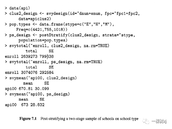
Example: Post-stratifying on school type.
In section 3.2 we examined a twostage sample drawn from the API population, with 40 school districts sampled from California and then up to five schools sampled from each district.
在第3.2节中,我们检查了从 API 人群中抽取的两阶段样本,从加利福尼亚抽取了40 个学区,然后从每个学区抽取了多达 5 个学校。
Post-stratifying this design on school type illustrates the situations where improvements in precision are and are not available.
在学校类型上对这种设计进行后分层说明了精度改进可用和不可用的情况。
The code and output are in Figure 7.1.
码和输出是在图7.1。
The first step is to set up the information about population group sizes.
第一步是设置有关人口群体大小的信息。
This information can be in a data frame (as here) or in a table object as is produced by the table() function.
此信息可以位于数据框(如此处)或由table()函数生成的表对象中。
In the data frame format, one or more columns give the values of the grouping variables and the final column, which must be named Freq, gives the population counts.
在数据框格式中,一列或多列给出分组变量的值,最后一列必须命名为 Freq,给出总体计数。
The call to poststratify() specifies the grouping variables as a model formula in the strata argument, and gives the table of population counts as the population argument.
对 poststratify() 的调用将分组变量指定为层参数中的模型公式,并给出人口计数表作为人口参数。
The function returns a new, post-stratified survey design object.
该函数返回一个新的、分层后的调查设计对象。
Post-stratification on school type dramatically reduces the variance when estimating total school enrollment across California.
在估计加利福尼亚州的总入学人数时,学校类型的后分层大大减少了差异。
The standard error was approximately 800,000 for the two-stage sample and less than 300,000 for the post-stratified sample.
两阶段样本的标准误约为800,000,分层后样本的标准误小于 300,000。
A large reduction in variance is possible because elementary schools are about half the size of middle schools and about one-third the size of high schools on average.
方差的大幅减少是可能的,因为平均而言,小学的规模约为中学的一半,约为高中的三分之一。
Post-stratification removes the component of variance that is due to differences between school types, and this component is large.
后分层去除了由于学校类型差异导致的方差分量,该分量很大。
When estimating the mean Academic Performance Index there is little gain from post-stratification.
在估计平均学业成绩指数时,分层后的收益很小。
A standardized assessment of school performance should not vary systematically by level of school or it would be difficult to interpret differences in scores.
学校表现的标准化评估不应因学校级别而有系统地变化,否则很难解释分数差异。
Since API has a similar mean in each school type, the between-level component of the variance is small and post-stratification provides little help.
由于 API 在每个学校类型中具有相似的平均值,因此方差的级别间分量很小,并且后分层提供的帮助很小。
If this were a real survey, non-response might differ between school type, and poststratification would then be useful in reducing non-response bias.
如果这是一次真正的调查,不答复可能因学校类型而异,而后分层将有助于减少不答复偏差。
7.3 RAKING
Post-stratification using more than one variable requires the groups to be constructed as a complete cross-classification of the variables.
使用多个变量的后分层需要将组构建为变量的完整交叉分类。
This may be undesirable: the cross-classification could result in so many groups that there is a risk of some of them not being sampled, or the population totals may be available for each variable separately, but not when cross-classified.
这可能是不可取的:交叉分类可能会导致如此多的组,以致于存在其中一些未被抽样的风险,或者每个变量的总体总数可能单独可用,但在交叉分类时不可用。
Raking allows multiple grouping variables to be used without constructing a complete cross-classification.
Raking 允许使用多个分组变量,而无需构建完整的交叉分类。
The process involves post-stratifying on each set of variables in turn, and repeating this process until the weights stop changing.
该过程包括依次对每组变量进行后分层,并重复此过程直到权重停止变化。
The name arises from the image of raking a garden bed alternately in each direction to smooth out the soil.
这个名字来源于在每个方向交替耙花园床以平整土壤的形象。
Raking can also be applied when partial cross-classifications of the variables are available.
当变量的部分交叉分类可用时,也可以应用倾斜。
For example, a sample could be alternately post-stratified using a two-way table of age and income, and a two-way table of sex and income.
例如,可以交替使用年龄和收入双向表以及性别和收入双向表对样本进行后分层。
The resulting raked sample would replicate the known population totals in both two-way tables.
由此产生的倾斜样本将在两个双向表中复制已知的总体总数。
The effect of matching observed and expected counts in lower-dimensional subtables is very similar to the effect of fitting a hierarchical loglinear model as described in section 6.3.1.
在低维子表中匹配观察到的和预期的计数的效果与拟合分层对数线性模型的效果非常相似,如第6.3.1节所述。
In fact, the raking algorithm is widely used to fit loglinear models, where it is known as iterative proportional jitting.
事实上,耙算法被广泛用于拟合对数线性模型,它被称为迭代比例抖动。
Raking could be considered a form of post-stratification where a loglinear model is used to smooth out the sample and population tables before the weights are adjusted.
Raking 可以被认为是一种后分层形式,在调整权重之前,使用对数线性模型来平滑样本和总体表。
Standard error computations after raking are based on the iterative post-stratification algorithm.
倾斜后的标准误差计算基于迭代后分层算法。
For standard errors based on replicate weights, raking each set of replicate weights ensures that the auxiliary information is correctly incorporated into between-replicate differences.
对于基于重复权重的标准误差,对每组重复权重进行倾斜可确保辅助信息正确地合并到重复之间的差异中。
For standard errors based on linearization, iteratively subtracting off stratum means in each direction gives residuals that incorporate the auxiliary information correctly.
对于基于线性化的标准误差,在每个方向上迭代地减去层均值会得到正确包含辅助信息的残差。
The rake () function performs the computations for raking by repeatedly calling poststratify().
耙()函数用于通过重复调用耙执行计算poststratify()。
Each of these calls to poststratify() accumulates the necessary information for standard error computations.
对poststratify() 的每一次调用都会为标准误差计算积累必要的信息。
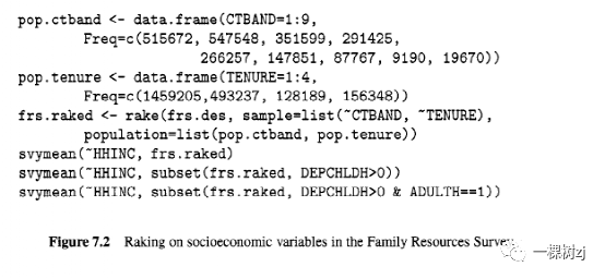
Example: Family Resources Survey,
In an example in Chapter 5 population data on council tax band and housing tenure in Scotland were used to fit a linear regression model to household income and improve the estimates of mean weekly income.
在第5章的一个例子中,苏格兰议会税收范围和住房使用权的人口数据被用来拟合家庭收入的线性回归模型,并改进对平均每周收入的估计。
Raking gives another way to use this information, and allows for estimation of mean weekly income in subpopulations as well as for the whole population.
Raking 提供了另一种使用此信息的方法,并允许估计子群体以及整个群体的平均每周收入。
Recall that in this example the weights have already been adjusted by raking before the data were provided, so that performing raking in R will not change the estimates, but will reduce the standard errors to the correct value.
回想一下,在这个例子中,在提供数据之前,权重已经通过倾斜进行了调整,因此在 R 中执行倾斜不会改变估计,但会将标准误差减少到正确的值。
The inputs to the rake() function are similar to those for postStratify(), except that a list of tables for each margin is specified rather than a single table.
rake()函数的输入与postStratify ()函数的输入类似,不同之处在于指定了每个边距的表格列表而不是单个表格。
Figure 7.2 has code for raking the survey design object defined in Figure 5.7.
图 7.2 具有用于倾斜图 5.7 中定义的调查设计对象的代码。
In this case we specify the population tables as two data frames.
在这种情况下,我们将人口表指定为两个数据框。
Each data frame has a variable with the same name as a raking variable in the survey design object and a variable Freq with population frequencies for the levels of this variable.
每个数据框都有一个与调查设计对象中的倾斜变量同名的变量和一个变量Freq ,该变量具有该变量水平的人口频率。
A list of two formulas specifies the names of the raking variables and a list of the two data frames (in the same order) specifies the population information.
两个公式的列表指定了倾斜变量的名称,两个数据框的列表(以相同的顺序)指定了人口信息。
Estimating mean household income for all households using the raked design object gives 2483 with standard error 27.5, the same as for the regression estimator and a substantial increase in precision over the standard error of 210.6 for the unraked design.
使用倾斜设计对象估计所有家庭的平均家庭收入为 2483,标准误差为 27.5,与回归估计量相同,并且精度比非倾斜设计的标准误差 210.6 显着提高。
Estimating the mean household income for all households with children gives 261 1, with a standard error of Ll2.5;
估计所有有孩子的家庭的平均家庭收入为 261 1,标准误为Ll2.5;
before raking the estimated mean was the same, but the standard error was 215.6.
在倾斜之前,估计平均值是相同的,但标准误差为 215.6。
The improvement in precision is almost non-existent for the smaller subpopulation of single-parent households, where the standard error of estimated mean weekly income is 28.5 before raking and 28.4 after raking.
对于较小的单亲家庭亚群,精确度的提高几乎不存在,其中估计平均每周收入的标准误差为耙前 28.5 和耙后 28.4。
This is partly because of the size of the subpopulation, and partly because the particular raking variables used here provide more detailed information about higher income levels.
这部分是因为亚群的规模,部分是因为这里使用的特定耙变量提供了关于更高收入水平的更详细信息。
For example, households with exactly two adults and two children make up about the same fraction of the population and of the sample as single-parent households, but the estimated mean weekly income for these households is 2714 with standard error 222.3 before raking and 2714 with standard error 219.7 after raking, a larger gain in precision.
例如,恰好有两个成人和两个孩子的家庭在人口和样本中与单亲家庭的比例大致相同,但这些家庭的估计平均每周收入为 2714,在抽佣前的标准误为 222.3,在抽佣前为 2714倾斜后的标准误差为 219.7,精度增益更大。
The benefit of raking decreases for smaller subpopulations because the full population information is less relevant to these smaller subgroups.
对于较小的亚群,耙集的好处会减少,因为完整的人口信息与这些较小的亚群不太相关。
In general, using population auxiliary information does not provide much extra precision in subpopulations unless the population information is specific to the subpopulations being analyzed.
一般而言,除非人口信息特定于正在分析的子人口,否则使用人口辅助信息不会在子人口中提供太多额外的精度。
Similar conclusions hold for the impact of raking on estimation of regression coefficients, as is illustrated in the next section.
类似的结论适用于耙对回归系数估计的影响,如下一节所示。
Chapter 8 looks at some examples where there is detailed auxiliary information specific to a particular regression model and useful gains in precision are realized.
第8章着眼于一些示例,其中包含特定于特定回归模型的详细辅助信息,并实现了对精度的有用增益。
In addition to allowing estimation of mean income in subpopulations, raking also allows the auxiliary information to be used in estimating other statistics, such as quantiles with svyquant ile ().
除了允许估计子总体中的平均收入外,耙还允许使用辅助信息来估计其他统计数据,例如带有 svyquantile () 的分位数。
In the original FRS design the estimated median weekly income was L355 with a 95% confidence interval L338-2372.
在最初的 FRS 设计中,估计的每周收入中位数为 L355,95% 的置信区间为 L338-2372。
After raking the 95% confidence interval is narrower: 23414369.
倾斜后,95% 的置信区间变窄:23414369。
7.4 generalized raking, greg estimation, and calibration
There are two related ways to view what is happening in post-stratification that allow extensions to continuous auxiliary variables and to a wide variety of other problems.
有两种相关的方法可以查看后分层中发生的情况,这些方法允许扩展到连续辅助变量和各种其他问题。
As in section 7.2, post-stratification can be seen as making the smallest possible changes to the weights that result in the estimated population totals matching the known totals.
如第 7.2 节所述,后分层可以被视为对权重进行尽可能小的更改,从而使估计的总体总数与已知总数相匹配。
This view of post-stratification leads to calibration estimators (Deville et al [41], Deville & Sarndal [40]).
这种分层后的观点导致了校准估计量(Deville 等人 [41]、Deville & Sarndal [40])。
An alternative is to note that the estimated population total after post-stratification is a regression estimator, for a working regression model that uses indicator variables for each post-stratum as predictors (see Exercise 7.5).
另一种方法是注意分层后的估计人口总数是一个回归估计量,对于使用每个后分层的指示变量作为预测变量的工作回归模型(参见练习 7.5)。
This view leads to generalized regression or GREG estimators (eg Sarndal et al [ 1521; Lehtonen and Veijanen[92]; Wu and Sitter[ 1901; Rao et al [ 1331) A thorough review of calibration is given by S h d a l [ 1491, who distinguishes between “calibration thinking” and “regression thinking” in constructing estimators using auxiliary information.
这种观点导致了广义回归或GREG估计量(例如 Sarndal 等 [ 1521;Lehtonen 和 Veijanen[92];Wu 和 Sitter[1901;Rao 等 [ 1331]) S hdal [ 1491,他在使用辅助信息构建估计量时区分“校准思维”和“回归思维”。
“Regression thinking” is useful in understanding why large increases in precision are possible - it is surprising to many biostatisticians that small changes in sampling weights can increase precision dramatically, but it is easier to understand that a good regression model can reduce the unexplained variation.
“回归思维”有助于理解为什么可以大幅提高精度——让许多生物统计学家感到惊讶的是,采样权重的微小变化可以显着提高精度,但更容易理解的是,一个好的回归模型可以减少无法解释的变化。
“Calibration thinking” often leads to simpler formulas and simpler software implementation, since an explicit model is not needed.
“校准思维”通常会导致更简单的公式和更简单的软件实现,因为不需要明确的模型。
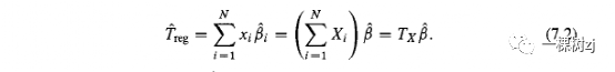
Given auxiliary variables Xi whose population totals Tx are known, the regression estimator of the population total was constructed in section 5.2.2.
给定总体总和Tx已知的辅助变量Xi ,在 5.2.2 节中构建了总体总和的回归估计量。
A regression model is fitted to the sample to obtain regression coefficients B and the estimated population total of Y is the population total of the fitted values
回归模型拟合样本以获得回归系数B ,Y的估计总体总数是拟合值的总体总数
The parameter estimates b from weighted least squares estimation can be written as a weighted sum of the sampled Yi, with weights depending on Xi and on the population totals of X .
来自加权最小二乘估计的参数估计b可以写成采样Yi的加权和,权重取决于Xi和X的总体总数。
This implies that TxB can also be written as a weighted sum of Y .
这意味着TxB也可以写成Y的加权和。
That, is
那是

for calibration weights gi that do not depend on Y.
对于不依赖于Y 的校准权重 gi 。
This is the calibration estimator of the population total.
这是总体总数的校准估计量。
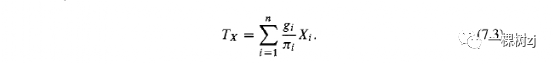
Because the weights do not depend on Y , they would be the same for estimating the population total of any variable, and in particular of X , so
因为权重不依赖于Y ,所以它们在估计任何变量的总体总数时是相同的,特别是X ,所以

Since a regression estimate of the population total of X that uses the known population total of X will be exactly correct, fp) = T x , and the calibration weights must satisfy the calibration constraints
由于使用X的已知总体总数的X总体总数的回归估计将完全正确,因此fp) = T x ,并且校准权重必须满足校准约束
The calibration weights gi make the estimated and known population totals agree.
校准权重gi使估计的和已知的总体总数一致。
If the Horvitz-Thompson estimate of T x is too small, gi will give more weight to large values of X ; if the Horvitz-Thompson estimate is too large, gi will downweight large values of X , When X and Y are correlated, the calibration weights that give exact estimation of TX will also give improved estimation of Ty .
如果T x的 Horvitz-Thompson 估计值太小,gi将给予较大的X值更多的权重;如果 Horvitz-Thompson 估计太大,gi将降低X 的大值,当X和Y相关时,给出TX精确估计的校准权重也将改进对Ty 的估计。
The calibration constraints in equation 7.3 do not uniquely define the weights.
等式 7.3 中的校准约束不唯一定义权重。
For example, if there is only one auxiliary variable X it is always possible to satisfy equation 7.3 by making a large change to the weight for just one observation.
例如,如果只有一个辅助变量X ,则总是可以通过对一次观测值进行较大的权重更改来满足等式 7.3 。
One way to completely specify gi is to also require that the calibrated weights are as close as possible to the sampling weights.
完全指定gi 的一种方法是还要求校准权重尽可能接近采样权重。
That is, for some distance function d ( , ), the calibration weights are chosen to make
也就是说,对于某个距离函数d ( , ),选择校准权重使

as small as possible while still satisfying the calibration constraints.
尽可能小,同时仍然满足校准约束。
The regression estimator of the population total corresponds to one choice of d ( , ) and the ratio estimator from section 5.1.3 to a different choice.
总体总体的回归估计量对应于d ( , ) 中的一个选择,而 5.1.3 节中的比率估计量对应于另一个选择。
Raking corresponds to the same choice of d ( , ) as ratio estimation.
Raking 对应于与比率估计相同的d ( , )选择。
In linear regression calibration, the calibration weights gi are a linear function of the auxiliary variables; in raking calibration the calibration weights are a multiplicative function of the auxiliary variables.
在线性回归校准中,校准权重gi是辅助变量的线性函数;在倾斜校准中,校准权重是辅助变量的乘法函数。
Ratio, raking, and regression estimators were already in widespread use before calibration was developed as a unifying description.
在校准被开发为统一描述之前,比率、倾斜和回归估计器已经被广泛使用。
The free choice of d ( , ) also allows new estimates to be constructed.
d ( , )的自由选择也允许构建新的估计。
The distance function can be chosen to force upper and lower bounds for g i , for example, specifying that gi > 0.5 and gi < 2, to prevent individual observations from becoming too influential and to prevent computational problems from zero or negative weights.
可以选择距离函数来强制gi 的上限和下限,例如,指定gi > 0.5 和gi < 2,以防止个别观察变得过于有影响力,并防止计算问题来自零或负权重。
The regression and calibration approaches to using auxiliary data do not always lead to the same estimates, but they do agree for a wide range of situations that arise frequently.
使用辅助数据的回归和校准方法并不总是导致相同的估计,但它们确实适用于经常出现的各种情况。
It is also worth noting that some of the situations where regression and calibration approaches differ according to Siirndal[ 1491 can be unified by considering regressions where the outcome variable is the individual contribution to a population equation.
还值得注意的是,根据 Siirndal[1491],回归和校准方法不同的一些情况可以通过考虑回归来统一,其中结果变量是个体对总体方程的贡献。
That is, “calibration thinking” can be duplicated by combining “regression thinking” with “influence function thinking”, as it has been in biostatistics.
也就是说,“校准思维”可以通过将“回归思维”与“影响函数思维”相结合来复制,就像在生物统计学中一样。
Calibration with influence functions is described in section 8.5.1 and details for the example given by Estevao and S h d a l are discussed in the Appendix, in section AS.
8.5.1 节描述了影响函数的校准,Estevao 和 S hdal 给出的例子的细节在附录的 AS 节中讨论。
Standard error estimates after calibration follow similar arguments to those for post-stratification.
校准后的标准误差估计遵循与分层后的类似论据。
When estimating a population total, a variable Yj can be decomposed into a true population regression value pi and a residual Yj - pi.
在估计总体总数时,变量Yj可以分解为真实的总体回归值pi和残差Yj - pi。
An unbiased estimator of variance of the estimated totals would be the Horvitz-Thompson variance estimator applied to Yi - pi.
估计总数的方差的无偏估计量是应用于Yi - pi的 Horvitz-Thompson 方差估计量。
Since pi is unknown, we apply the Horvitz-Thompson estimator to Yi - pi and obtain a variance estimator that is nearly unbiased as long as the number of parameters in the regression model is not too large (Siirndal et al.[152]).
由于pi未知,我们将 Horvitz-Thompson 估计量应用于Yi - pi并获得几乎无偏的方差估计量,只要回归模型中的参数数量不太大(Siirndal 等人 [152])。

When estimating other statistics the residuals are taken after linearization, as described in Appendix C.l.
当估计其他统计量时,在线性化后采用残差,如附录 C 中所述
As usual, the estimation is more straightforward with replicate weights.
像往常一样,使用重复权重进行估计更直接。
Once the calibration procedure is applied to each set of replicate weights, the variances then automatically incorporate the auxiliary information.
一旦校准程序应用于每组重复权重,方差就会自动包含辅助信息。
7.4.1 Calibration in R
The survey package provides calibration with the calibrate() function.
survey包提供校准与calibrate()函数。
As with poststratify() and rake(), this function takes a survey design object as an argument and returns an updated design object with adjusted weights and all the necessary information to compute standard errors.
与 poststratify() 和 rake() 一样,此函数将调查设计对象作为参数,并返回具有调整权重和所有必要信息以计算标准误差的更新设计对象。
The auxiliary variables are specified using a model formula, as for post-stratification, and the population totals are specified as the column sums of the population regression design matrix (predictor matrix) corresponding to the model formula.
辅助变量使用模型公式指定,对于后分层,人口总数指定为模型公式对应的人口回归设计矩阵(预测矩阵)的列总和。
Linear regression calibration.
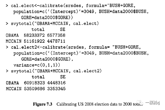
Figure 7.3 uses calibration to repeat the estimates of US 2008 presidential election totals from Figure 5.8.
图7.3使用校准来重复图 5.8 中对美国 2008 年总统选举总数的估计。
The auxiliary variables are the votes in the 2000 election for George W. Bush and A1 Gore.
辅助变量是 2000 年 George W. Bush 和 A1 Gore 的选票。
The formula argument specifies the auxiliary variables, and the population argument gives the population totals.
公式参数指定辅助变量,人口参数给出人口总数。
In this example there are population totals for the intercept, and for the variables BUSH and GORE - the intercept is always included implicitly.
在这个例子中,截距有人口总数,对于变量 BUSH 和 GORE -截距总是隐式地包括在内。
In Figure 5.8 separate regression models were needed to estimate totals for Obama and McCain.
在图 5.8 中,需要单独的回归模型来估计奥巴马和麦凯恩的总数。
Calibrating the survey design object incorporates the auxiliary information in all estimates, so the totals for both candidates can simply be estimated with svytotal() .
校准调查设计对象会在所有估计中包含辅助信息,因此可以使用 svytotal() 简单地估计两个候选人的总数。
The second call to calibrate() specifies a different distance function d( , ), one that is optimal when the variability in Y is proportional to the calibration variables.
对calibration() 的第二次调用指定了一个不同的距离函数d( , ),当Y 的可变性与校准变量成比例时,该函数是最佳的。
In this case, the vector c (0, I , 1) specifies calibration weights that would be optimal if the variance of Y is proportional to 1 x BUSH + 1 x OBAMA, i.e., to the number of votes.
在这种情况下,如果 Y 的方差与 1 x BUSH + 1 x OBAMA(即投票数)成正比,向量 c (0, I, 1) 指定了最佳校准权重。
This calibration gives very similar results to the regression estimators of totals using the working model with variance proportional to mean in Figure 5.8.
这种校准给出了与使用方差与均值成正比的工作模型的总数回归估计器非常相似的结果,如图 5.8 所示。
The results would be identical if the coefficients from the regression models in Figure 5.8 were used in the variance argument.
如果在方差参数中使用图 5.8 中回归模型的系数,结果将是相同的。
Raking calibration.
Repeating the example of raking from the Family Resources Survey (Figure 7.2) using the calibrate() function gives the code in Figure 7.4.
使用calibrate() 函数重复从家庭资源调查(图7.2)中抽取的示例,得到图7.4 中的代码。
In a regression model the two factor variables CTBAND and TENURE would be coded as an intercept and an indicator variable for each category except the first.
在回归模型中,两个因子变量 CTBAND 和 TENURE 将被编码为除第一个之外的每个类别的截距和指示变量。
The population total for the intercept is the population size, and this is concatenated with the counts for each of the auxiliary variables, dropping the first category of each.
截距的人口总数是人口规模,它与每个辅助变量的计数连接在一起,去掉每个辅助变量的第一个类别。
The option calfun="raking" requests the calibration distance function that is equivalent to raking.
选项 calfun="raking" 请求等效于 raking 的校准距离函数。
The estimates of mean (and median) weekly income based on the calibrated design are identical to those obtained from the raked design in Figure 7.2.
基于校准设计的平均(和中位数)周收入估计值与从图 7.2 中的倾斜设计中获得的估计值相同。
The advantage of raking calibration using calibrate() over raking using rake () is that calibrate() can use continuous auxiliary variables and rake() can use only discrete variables.
使用calibration() 进行倾斜校准比使用rake() 进行倾斜的优点在于,calibrate() 可以使用连续辅助变量,而rake() 只能使用离散变量。
Logit calibration and bounded weights.
A popular calibration function in Europe gives so-called logit calibration.
欧洲流行的校准函数提供所谓的 logit 校准。
This distance function requires the user to specify upper and lower bounds on the calibration weights.
此距离函数要求用户指定校准权重的上限和下限。
If possible, the calibrate() will return calibration weights that satisfy the bounds.
如果可能,calibrate() 将返回满足边界的校准权重。
It may be impossible to satisfy both the bounds and the calibration constraints (Equation 7.3),
可能无法同时满足边界和校准约束(公式 7.3),
in which case calibrate() will give an error.
在这种情况下,calibrate() 会出错。
The force=TRUE option forces calibrate() to return a survey design in which the weights satisfy the bounds even if the calibration constraints are not met.
force=TRUE 选项强制calibrate()返回一个测量设计,其中即使不满足校准约束,权重也满足边界。
This is useful to allow a series of simulations to be completed, and may be useful for data analysis if the calibration constraints are nearly met, which can be easily checked using svytota() .
这对于允许完成一系列模拟很有用,如果几乎满足校准约束,则可能对数据分析有用,这可以使用 svytota ()轻松检查。
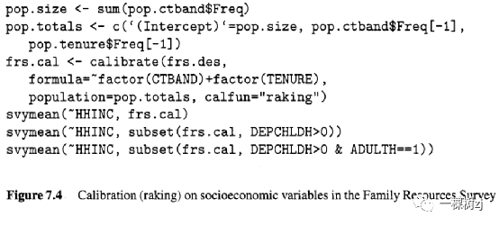
Figure 7.5 shows code for logit calibration on a cluster sample of school districts from the Academic Performance Index population.
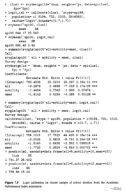
图 7.5 显示了对来自学业成绩指数人群的学区集群样本进行 logit 校准的代码。
Using linear calibration with the same auxiliary variables gives calibration weights ranging from 0.4 to 1.8, with logit calibration the weights vary from slightly above the lower bound of 0.7 to slightly below the upper bound of 1.7.
使用具有相同辅助变量的线性校准,校准权重范围从 0.4 到 1.8,使用 logit 校准,权重从略高于 0.7 的下限到略低于 1.7 的上限变化。
Calibration using the 1999 Academic Performance Index gives a dramatic reduction in standard error for estimating the mean of the 2000 Academic Performance Index.
使用 1999 年学业成绩指数进行校准可显着降低估计 2000 年学业成绩指数平均值的标准误差。
In a regression model with Academic Performance Index as the outcome there is a substantial increase in precision for the intercept but not for the slope estimates.
在以学业成绩指数作为结果的回归模型中,截距的精度显着提高,但斜率估计的精度没有显着提高。
In this model the predictors are proportion of "English Language Learners" ( e l l ) , proportion of students who are new to the school (mobility) and proportion of teachers with only emergency qualifications (emer).
在这个模型中,预测变量是“英语学习者”的比例( ell )、新到学校的学生比例(流动性)和只有紧急情况资格的教师比例( emer )。
These predictors and the outcome are quite strongly associated with the auxiliary variables, but this is not enough to give an increase in precision for comparisons across levels of the predictors.
这些预测变量和结果与辅助变量有很强的相关性,但这不足以提高跨预测变量水平比较的精度。
The problem of calibration to increase precision for coefficient estimates in regression models is discussed further in Chapter 8.
第8章进一步讨论了校准以提高回归模型中系数估计的精度的问题。
Gains in precision are possible, but they require calibration targeted to the specific model.
提高精度是可能的,但它们需要针对特定模型进行校准。
Calibration of large surveys carried out when the data is collected is not likely to increase precision for regression models fitted in secondary data analysis.
在收集数据时进行的大型调查的校准不太可能提高二次数据分析中拟合的回归模型的精度。
On the other hand, the reduction in uncertainty for the intercept can (and in this example does) translate to a useful reduction in standard errors for fitted values.
另一方面,截距不确定性的降低可以(在本例中确实如此)转化为拟合值标准误差的有用降低。
Comparing calibration methods.
比较校准方法。
In the absence of non-response, the choice of calibration function makes little difference to the resulting estimated totals, with the difference decreasing as sample size increases [40].
在没有无响应的情况下,校准函数的选择对所得估计总数几乎没有影响,差异随着样本量的增加而减小 [40]。
In finite samples or with nonresponse it is possible for the results to differ, but they typically do not.
在有限样本或无响应情况下,结果可能会有所不同,但通常不会。
Kalton and Flores-Cervantes [69] gave an artificial example of calibration comparing a range of calibration methods.
Kalton 和 Flores-Cervantes [69] 给出了一个人工校准示例,比较了一系列校准方法。
Code to reproduce their analyses is in the tests subdirectory of the survey package, in the file kalton.
重现他们的分析的代码位于survey包的测试子目录中的文件kalton 中。
Rand Figure 7.6 shows some of the resulting sets of calibration weights.
Rand 图 7.6 显示了一些校准砝码的结果集。
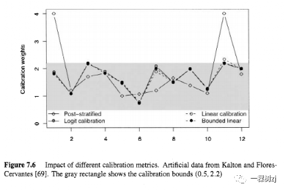
The data form a 3 x 4 table and there are three sets of calibration weights using the margins of the table, and the set resulting from poststratification on the cells of the table.
数据形成一个3 x 4 表格,有三组使用表格边缘的校准权重,以及由表格单元格上的后分层产生的集合。
The three sets of weights based on the margins of the table use linear calibration, logit calibration, and bounded linear calibration, with both logit and bounded linear calibration having a lower bound of 0.5 and an upper bound of 2.2, as indicated by the shaded region.
三组基于表边距的权重使用线性校准、logit校准和有界线性校准,logit和有界线性校准的下限为0.5,上限为2.2,如阴影区域所示.
The two bounded techniques give weights inside the shaded region; linear calibration gives one weight slightly outside the region at 2.34.
这两种有界技术在阴影区域内给出权重;线性校准在 2.34 的区域外给出一个权重。
It is clear from the graph that the choice of auxiliary variables is much more important than the choice of calibration function.
从图中可以看出,辅助变量的选择比校准函数的选择重要得多。
The three sets of weights using the margins of the table are very similar, and are quite different from the weights using all the cell counts in the table.
使用表格边距的三组权重非常相似,与使用表格中所有单元格计数的权重有很大不同。
Adding additional calibration variables will always give increased precision (or reduced non-response bias) with sufficiently large sample sizes, but for any given sample size there will be a point where the added uncertainty from estimating parameters in the calibration model outweighs the gains.
添加额外的校准变量总是会在样本量足够大的情况下提高精度(或减少无响应偏差),但对于任何给定的样本量,都会有一个点,即校准模型中估计参数所增加的不确定性会超过收益。
Judkins et al [68] describe one approach to assessing whether added auxiliary variables are helpful.
Judkins 等人 [ 68]描述了一种评估添加的辅助变量是否有用的方法。
Cluster-level weights.
When the last stage of a probability design involves cluster sampling, such as sampling all individuals in a household, the sampling weights for individuals in the same cluster are necessarily identical.
当概率设计的最后阶段涉及聚类抽样时,例如对家庭中的所有个人进行抽样,同一聚类中个人的抽样权重必然相同。
Especially for official statistics, it may be desirable for the calibrated weights for individuals in the same cluster to also be identical.
特别是对于官方统计数据,可能希望同一集群中个人的校准权重也相同。
This provides internal consistency between estimates, though at a small cost in efficiency.
这提供了估计之间的内部一致性,但效率成本很小。
For example, in collecting data on a sample of births, where every infant must have exactly one mother, it would be undesirable for estimated subpopulation totals of mothers to add up to more than the estimated total number of infants.
例如,在收集有关出生样本的数据时,每个婴儿必须只有一个母亲,估计母亲亚群总数的总和超过估计的婴儿总数是不可取的。
The aggregate.stage argument to calibrate() specifies the stage of sampling at which calibration weights must be constant within clusters.
calibrate()的aggregate.stage参数指定采样阶段,在该阶段校准权重必须在集群内保持不变。
This argument is available only for survey design objects that include the sampling design.
此参数仅适用于包含抽样设计的调查设计对象。
For survey design objects based on replicate weights the aggregate.index argument specifies a vector of cluster identifiers so that calibration weights will be made equal within the same cluster.
对于基于重复权重的调查设计对象,aggregate.index参数指定集群标识符向量,以便在同一集群内使校准权重相等。
As an example, consider the two-stage cluster sample from Academic Performance Index population.
例如,考虑来自学业成绩指数总体的两阶段聚类样本。
The first stage of the design samples school districts and the second stage samples up to five schools within each district.
设计的第一阶段对学区进行抽样,第二阶段对每个区内最多五所学校进行抽样。
Sampling probabilities, and thus sampling weights, are the same for schools within the same school district.
同一学区内的学校的抽样概率和抽样权重是相同的。
When the sample was post-stratified on school type in Figure 7.1 the calibration weights were not the same for schools within the same cluster, varying up to 20% between school type.
当样本按图 7.1 中的学校类型进行后分层时,同一集群内的学校的校准权重不同,学校类型之间的差异高达 20%。
In Figure 7.7 the weights are forced to be constant within a school district, that is, within each stage-1 sampling unit.
在图 7.7 中,权重在学区内,即在每个阶段 1 抽样单位内被迫保持不变。
There is a slight cost in precision, with the standard error for the estimated total enrollment increasing by about 20%.
精确度略有成本,估计总入学人数的标准误差增加了约 20%。
This loss of precision occurs because the weights become more variable across school districts to compensate for the added constraints.
出现这种精度损失是因为权重在各学区之间变得更加可变,以补偿增加的约束。
The calibration weights in the simple post-stratified design range from 1.08 to 1.27, with constant weights within school district the range is from 0.64 to 1.68.
简单后分层设计中的校准权重范围为 1.08 至 1.27,学区内的恒定权重范围为 0.64 至 1.68。
It is also possible to do the converse: to use auxiliary information where population totals are available only for sampled clusters at some stage of sampling, not for the whole population.
也可以反过来:使用辅助信息,其中总体总数仅适用于某个抽样阶段的抽样集群,而不适用于整个总体。
This is done by supplying a list of population totals for the sampled clusters, with the names on the list matching the cluster identifiers, and giving the stage argument to calibrate() to indicate which stage of sampling the totals belong to.
这是通过提供抽样集群的总体总数列表来完成的,列表中的名称与集群标识符匹配,并将阶段参数提供给校准()以指示总数属于哪个抽样阶段。
An example using the same two-stage sample from the Academic Performance Index population is given in the t e s t s subdirectory of the survey package, in the file caleg.R.
survey包的测试子目录中的文件 caleg 中给出了使用来自学业成绩指数总体的相同两阶段样本的示例。R。
7.5 basu's elephants
Basu [3, 971 gave an example that was intended to show unreasonable behavior of design-based inference, but that can be interpreted in terms of poor use of auxiliary information.
Basu [3, 971 给出了一个例子,该例子旨在展示基于设计的推理的不合理行为,但可以解释为辅助信息使用不当。
In his story a circus owner had 50 elephants and wanted an estimate of their total weight based on weighing only one elephant.
在他的故事中,一个马戏团老板有 50 头大象,想要根据只称一头大象的重量来估计它们的总重量。
In the absence of any additional information a sensible approach would be to take a simple random sample of one elephant and weigh it (El), and then multiply by the sampling weight.
在没有任何附加信息的情况下,一种明智的方法是从一头大象中抽取一个简单的随机样本并对其进行称重 (El),然后乘以采样权重。
This is a valid design-based estimate, although no unbiased estimate of the standard error is available from a sample of size one.
这是一个有效的基于设计的估计,尽管无法从大小为 1 的样本中获得标准误差的无偏估计。
The circus owner knows that five years previously, when all the elephants were last weighed, a particular mid-sized elephant, Sambo, had very nearly the average weight.
马戏团老板知道,五年前,当所有大象最后一次称重时,一头中型大象 Sambo 的体重非常接近平均体重。
A reasonable model-based estimate of the total weight of the elephants now would be
一个大象的总重量的合理的基于模型的估计现在会是
This is not a valid design-based estimate; no unbiased design-based estimate can be obtained when the sampling probabilities are zero for 49 of 50 elephants.
这不是基于设计的有效估算;当 50 头大象中的 49 头的抽样概率为零时,无法获得基于设计的无偏估计。
Basu imagines a compromise design worked out between the circus owner and the circus statistician, in which Sambo is sampled with very high probability (rsarnb= 0.99) and the remaining probability is divided up among the other elephants (ni = 1/5000).
Basu 设想了一种在马戏团老板和马戏统计员之间制定的折衷设计,其中 Sambo 以非常高的概率 (rsarnb = 0.99)进行采样,剩余的概率在其他大象之间分配(ni = 1/5000)。
When the sampling is performed, Sambo is in fact chosen.
执行采样时,实际上选择了 Sambo。
The circus owner expects the estimate to be 50 x ESambo, but the statistician points out that the Horvitz-Thompson estimator is
马戏团老板预计估计值为 50 x ESambo,但统计学家指出 Horvitz-Thompson 估计值为
This estimate is clearly silly.
这个估计显然是愚蠢的。
Worse still, if one of the other elephants, e g , the largest elephant, Jumbo, had been weighed, the Horvitz-Thompson estimator would be
更糟糕的是,如果对其他大象之一(例如最大的大象 Jumbo)进行称重,则 Horvitz-Thompson 估计量将是
 The Horvitz-Thompson estimator is exactly unbiased, but this is a property defined by averaging over possible realizations of the sampling design.
Horvitz-Thompson 估计量是完全无偏的,但这是通过对抽样设计的可能实现求平均来定义的属性。
For any single realization of the sampling design the result will be clearly unreasonable.
对于抽样设计的任何单一实现,结果显然是不合理的。
This example is somewhat embarrassing for design-based inference, so it is worth considering why such poor results are obtained.
这个例子对于基于设计的推理来说有些尴尬,所以值得思考为什么会得到如此糟糕的结果。
To some extent the unreasonable result is the fault of the small sample.
不合理的结果在某种程度上是小样本的错。
In large samples we can be confident that the value of an estimate will be close to its expected value, so it is useful to know that the expected value is equal to the true population value.
在大样本中,我们可以确信估计值将接近其期望值,因此知道期望值等于真实总体值是有用的。
In small samples, where an estimate need not be close to the expected value, unbiasedness is not sufficient to ensure reasonable behaviour.
在小样本中,估计不需要接近预期值,无偏性不足以确保合理的行为。
However, the Horvitz-Thompson estimate is supposed to be useful even in small samples, so something is still wrong.
然而,即使在小样本中,Horvitz-Thompson 估计也应该是有用的,所以仍然存在一些问题。
The first question is whether the “compromise” design is actually a sensible use of the prior knowledge if the Horvitz-Thompson estimator is going to be used.
第一个问题是,如果要使用 Horvitz-Thompson 估计量,“妥协”设计是否实际上是对先验知识的明智使用。
The second question is whether the Horvitz-Thompson estimator is appropriate, given the auxiliary information that is available.
第二个问题是,考虑到可用的辅助信息,Horvitz-Thompson 估计量是否合适。
The answer to both questions is “No”.
这两个问题的答案都是“否”。
Using auxiliary information in design.
在设计中使用辅助信息。
In choosing which elephant to weigh it is helpful to consider a situation where the sample size is slightly larger.
在选择要称重的大象时,考虑样本量稍大的情况是有帮助的。
If the circus were weighing three elephants rather than one, they could consider stratified sampling.
如果马戏团称重三头大象而不是一头,他们可以考虑分层抽样。
Equation 2.6 in section 2.6 gives the optimal allocation: proportional to the number in each stratum and to the standard deviation in the stratum.
第 2.6 节中的公式 2.6 给出了最佳分配:与每个层中的数量和层中的标准偏差成正比。
If the elephants were divided into small, medium, and large by eye (or by previous weight), taking one elephant at random from each stratum would make sense.
如果将大象按眼睛(或以前的体重)分为小、中、大,那么从每个层随机抽取一头大象就有意义了。
This leads to reasonable estimates and makes use of available information.
这会导致合理的估计并利用可用信息。
A stratified sampling approach would lead to sampling probabilities ni that did not vary much between elephants.
一个分层抽样方法会造成采样概率妮未大象之间变化不大。
A similar approach, ranked-set sampling [72,107,123], is used in some ecological applications.
甲类似的方法,排集采样[72107123],在一些生态应用中。
Three samples of three elephants would be taken at random, and the elephants in each sample ranked by size.
将随机抽取三头大象的三个样本,每个样本中的大象按大小排列。
The smallest elephant from the first sample, the middle elephant from the second sample, and the largest elephant from the third sample are weighed.
对第一个样本中最小的大象、第二个样本中的中间大象和第三个样本中的最大大象进行称重。
The ranking procedure has a similar effect to stratification, but ranking is often easier - lining up all the elephants by size would be more work than judging which of three is largest.
排序过程与分层有类似的效果,但排序通常更容易-按大小排列所有大象比判断三个中哪一个最大要多。
Under ranked-set sampling the sampling weight ni is the same for every unit in the population.
在排序集抽样下,抽样权重ni对于总体中的每个单元都是相同的。
Section 3.3 considered sampling clusters proportional to size, or more generally, sampling observations proportional to some auxiliary variable available for the whole population.
第 3.3 节考虑了与规模成正比的抽样集群,或更一般地说,抽样观察与整个总体可用的某些辅助变量成正比。
If the sampling probabilities are roughly proportional to the variable being analyzed, the variance of the estimated total will be small.
如果抽样概率与被分析的变量大致成正比,则估计总数的方差将很小。
In applying this principle to the elephants the circus owner could use either the weights recorded at the previous weighing, or if these are lost, an approximate measure of elephant volume as height x length x width.
在将这一原则应用于大象时,马戏团老板可以使用上次称重时记录的重量,或者如果这些重量丢失,则可以使用大象体积的近似度量,如高x长x宽。
Under this PPS sampling scheme the sampling probability would be highest for the largest elephant.
在这种PPS抽样方案下,最大的大象的抽样概率最高。
The variation between elephants in sampling probabilities would still be much smaller than for Basu’s design, since the record weight for an elephant is only about twice the typical adult weight.
大象之间在抽样概率方面的差异仍然比 Basu 的设计小得多,因为一头大象的创纪录体重仅为典型成年体重的两倍左右。
Based on the standard techniques used for designing complex samples it appears that if the Horvitz-Thompson estimator were to be used in analysis, a good design would have much less variation in sampling probabilities than Basu’s design and that sampling larger elephants with modestly higher probability would be helpful.
根据用于设计复杂样本的标准技术,似乎如果在分析中使用 Horvitz-Thompson 估计量,那么好的设计在抽样概率方面的变化会比 Basu 的设计小得多,并且以适度更高的概率对较大的大象进行抽样会乐于助人。
Using auxiliary information in analysis.
在分析中使用辅助信息。
A better way to use auxiliary information about the elephants would be by some form of calibration.
一个更好的方式来使用辅助信息有关的大象会通过某种形式的校准。
For example, calibrating the estimated population size N = l/ni to the known population size N = 50 gives calibrated weights gi /Ti = 50. The resulting model-assisted estimate of the total is
例如,将估计的总体规模N = l/ni校准到已知的总体规模N = 50 给出校准权重gi /Ti = 50。由此产生的模型辅助估计总数为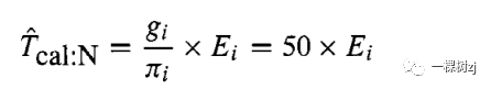
Two solutions to the calibration constraints are
校准约束的两种解决方案是
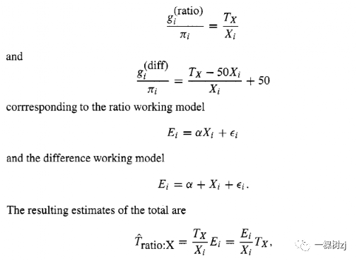
where the previous total is multiplied by the relative increase in weight for the measured elephant, and
其中先前的总数乘以权重的相对增加测量大象,和
where 50 times the absolute increase in weight for the measured elephant is added to the previous total.
其中 50 倍的被测大象的重量绝对增加被添加到之前的总数中。
These estimators are likely to be more precise than the Horvitz-Thompson estimator because they only need to estimate the relatively small change in weight since the previous weighing.
这些估计量可能比 Horvitz-Thompson 估计量更精确,因为它们只需要估计自上次称量以来相对较小的重量变化。
Using these estimators it is no longer desirable to sample Sambo with higher probability, in contrast to f c a l : ~b, e cause the auxiliary information is already being used efficiently.
与 fcal 相比,使用这些估计器不再需要以更高的概率对 Sambo 进行采样:~b,e 因为辅助信息已经被有效地使用了。
The fact that only one elephant is weighed limits the choice of working models to the simple ratio and difference models.
仅称重一头大象的事实将工作模型的选择限制为简单的比率和差异模型。
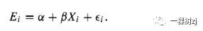
If the circus owner had wanted to weigh five elephants out of 250 it would be possible to do better using a working model with more parameters, such as
如果马戏团老板想称重 250 头大象中的 5 头,那么使用具有更多参数的工作模型可能会做得更好,例如
This analysis shows that the circus statistician’s failure in Basu’s example was not adherence to design-based inference but ignorance of calibration estimators as the appropriate way to use auxiliary information.
该分析表明,马戏团统计学家在 Basu 的例子中的失败不是坚持基于设计的推理,而是无视校准估计量作为使用辅助信息的适当方式。
It is true that some of the approaches described here use more information than just the fact that
确实,这里描述的一些方法使用了更多的信息,而不仅仅是这样一个事实
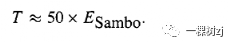
If the circus owner knew that this was a sufficiently accurate approximation it would obviously be sensible just to weigh Sambo, but it is hard to imagine being sure of this without knowing anything else.
如果马戏团老板知道这是一个足够准确的近似值,那么仅称三宝显然是明智的,但很难想象在不知道其他任何事情的情况下确定这一点。
For example, it is hard to imagine how the owner would know that the weight gains of the elephants over the past five years add up to 50 times Sambo’s weight gain without also knowing that, e.g., the weight gains have been similar for each elephant.
例如,很难想象主人在不知道例如每头大象的体重增加相似的情况下,如何知道过去五年大象的体重增加加起来是三宝体重增加的50倍。
The point of this example is not to argue that design-based estimates are to be preferred to model-based estimates, but to show that when a design-based estimate gives a clearly inappropriate estimate it is probably because it is not a good designbased estimate.
这个例子的重点不是争辩说基于设计的估计比基于模型的估计更受欢迎,而是表明当基于设计的估计给出明显不合适的估计时,可能是因为它不是一个好的基于设计的估计.
7.6 selecting auxiliary variables for non-response
7.6 选择无响应的辅助变量
Post-stratification, raking, and calibration are widely used to reduce the bias from unit non-response, people who cannot be contacted or refuse to participate in surveys.
后分层、倾斜和校准被广泛用于减少单位不响应、无法联系或拒绝参与调查的人的偏差。
This problem is increasing over time, especially for telephone surveys; the University of Michigan’s Survey of Consumer Attitudes found response rates decreasing by about 1% per year from 1979 to 2003 (Curtin et al. citecurtin-nonresponse), and the response rate in the Behavioral Risk Factor Surveillance System declined from about 70% in 1991 to about 50% in 2001.
这个问题随着时间的推移而增加,特别是对于电话调查;密歇根大学的消费者态度调查发现,从 1979 年到 2003 年,响应率每年下降约 1%(Curtin 等人,citcurtin-nonresponse),行为风险因素监测系统的响应率从 1991 年的约 70% 下降2001 年达到 50% 左右。
Reweighting for non-response is not a purely design-based method; it relies implicitly on models for the missing data.
对无响应重新加权并不是一种纯粹基于设计的方法;它隐含地依赖于缺失数据的模型。
In the simplest case, post-stratification, the model is that non-response is independent of the outcome variable within groups defined by the auxiliary variables.
在最简单的情况下,后分层,模型是无响应独立于由辅助变量定义的组内的结果变量。
For example, suppose the probability of responding to a telephone survey about health insurance was higher for landline than cellphone users but within each group the probability of responding was independent of whether the individual had health insurance.
例如,假设固定电话用户回答有关健康保险的电话调查的概率高于手机用户,但在每个组中,回答的概率与个人是否有健康保险无关。
An estimate using sampling weights based on the design would give too little weight to cellphone users (who tend to be younger) and so would be biased.
使用基于设计的抽样权重的估计会给手机用户(往往更年轻)提供太少的权重,因此会产生偏差。
If the telephone companies could be persuaded to give population numbers of landline and cellphone numbers, the analysis could be post-stratified by telephone type to give a valid estimate.
如果可以说服电话公司提供固定电话和手机号码的人口数量,则可以按电话类型对分析进行后分层以给出有效估计。
This example also illustrates some of the limits of non-response adjustment: no reweighting, however sophisticated, will allow a telephone survey to give information about people without telephone service.
这个例子也说明了不答复调整的一些限制:没有重新加权,无论多么复杂,都将允许电话调查提供有关没有电话服务的人的信息。
One way to look at the effect of post-stratification is that the correct sampling probability for a homogenous group of people is not the intended probability ti but the achieved probability.
查看后分层效果的一种方法是,同质人群的正确抽样概率不是预期概率ti,而是实现概率。
If we try to sample 100 women aged 25-35 from a population of 10,000 and only 76 of them respond, the actual sampling fraction is not 100/10,000 but 76/10,000.
如果我们尝试从 10,000 人中抽取 100 名 25-35 岁的女性,而其中只有 76 人做出回应,那么实际抽样比例不是 100/10,000,而是 76/10,000。
This correction is exactly what post-stratification does
这种修正正是后分层所做的
There are two relevant ways that a group can be homogenous.
有两种相关方式可以使组同质化。
If the non-response probability is homogenous within the group, as above, then post-stratification will give correct sampling weights, in the sense that the population total for any variable is correctly estimated.
如果组内的无响应概率是同质的,如上所述,则后分层将给出正确的抽样权重,即任何变量的总体总数都被正确估计。
On the other hand, if a particular outcome variable is homogenous within the group, the population total for that outcome variable will be correctly estimated even if response is not homogenous: the relative weighting for individuals within the group will be wrong, but as the outcome is the same this incorrect relative weighting does not matter.
另一方面,如果特定的结果变量在组内是同质的,即使响应不是同质的,该结果变量的总体总数也将被正确估计:组内个体的相对权重将是错误的,但作为结果是一样的,这个不正确的相对权重无关紧要。
More generally, if a regression model using the auxiliary variables can explain most of the variation in an outcome, the residual variation will be small and bias in analyzing it will be small in absolute terms even if large in relative terms.
更一般地说,如果使用辅助变量的回归模型可以解释结果中的大部分变化,则残差变化将很小,并且分析它的偏差在绝对方面也很小,即使相对而言很大。
These two possibilities are analogous to the two constructions of calibration by “regression thinking” and “calibration thinking” in section 7.4.
这两种可能性类似于7.4节中“回归思维”和“校准思维”的两种校准结构。
1, For large-scale surveys there are usually only a small number of possible auxiliary variables and the goal must be to be produce correct results for all analyses, not just for a few chosen variables, so homogeneity of response is much more important.
1、对于大规模调查,通常只有少量可能的辅助变量,目标必须是为所有分析产生正确的结果,而不仅仅是针对少数选定的变量,因此响应的同质性更为重要。
Of course, there is no realistic prospect of achieving true homogeneity of response using the few auxiliary variables typically available, but the estimates after poststratification are probably less biased than those before post-stratification.
当然,使用通常可用的少数辅助变量来实现响应的真正同质性是不现实的,但后分层后的估计可能比后分层前的估计偏差更小。
Keeter et al [73] published results from an encouraging experiment that administered the same questionnaire in two telephone surveys, one of which made very extensive efforts to reduce non-response.
Keeter 等人 [73] 发表了一项令人鼓舞的实验结果,该实验在两次电话调查中使用相同的问卷调查,其中一次为减少不答复做出了非常广泛的努力。
The non-response rates were 36% and 60% for the two surveys.
两项调查的不答复率分别为 36% 和 60%。
Even before any form of reweighting, the differences in political and social attitudes between responders to the two surveys wer much smaller than the differences in demographic variables.
即使在进行任何形式的重新加权之前,两项调查的受访者之间的政治和社会态度差异也远小于人口统计变量的差异。
This shows that even quite high levels of non-response in an otherwise well-conducted survey may still give reasonable results.
这表明,即使在进行良好的调查中出现相当高的不答复水平,也可能会给出合理的结果。
It also suggests that post-stratification or calibration should work well, since the demographic variables most likely to be used for reweighting the sample appeared more sensitive to response rates than the outcome variables being studied.
它还表明后分层或校准应该运作良好,因为最有可能用于重新加权样本的人口统计变量似乎比正在研究的结果变量对响应率更敏感。
7.6.1 Direct standardization
7.6.1 直接标准化
Direct standardization of rates is the term used in epidemiology and demography for reweighting a sample from one population so that the distribution of variables such as age group and sex matches a different population.
比率的直接标准化是流行病学和人口学中使用的术语,用于重新加权来自一个群体的样本,以便年龄组和性别等变量的分布与不同的群体相匹配。
Direct standardization is used either to extrapolate to an estimate of the rate in the target population or to compare the extrapolated rate to the observed rate in the target population.
直接标准化用于外推到目标人群中的比率估计值,或将外推的比率与目标人群中观察到的比率进行比较。
For example, comparing the outcomes of neonatal care in different hospitals is difficult because the hospitals may have different numbers of high-risk, low birth weight infants.
例如,比较不同医院新生儿护理的结果很困难,因为医院可能有不同数量的高危、低出生体重婴儿。
Direct standardization for birthweight allows a comparison based on the same distribution of birth weight in different hospitals.
出生体重的直接标准化允许基于不同医院出生体重的相同分布进行比较。
Post-stratification for non-response and direct standardization are mathematically equivalent, but post-stratification is usually done with the intention of getting an improved estimate in the target population, and direct standardization is more often done to compare the known rates in the target population with rates extrapolated from the source sample.
无响应的后分层和直接标准化在数学上是等效的,但后分层通常是为了在目标人群中获得改进的估计值,而直接标准化更常用于比较目标人群中的已知比率与从源样本外推的比率。
That is, post-stratification for non-response relies on the assumption that category-specific rates will be the same in the sample and target population, where direct standardization is often used to evaluate whether or not the category-specific rates are the same.
也就是说,不答复的后分层依赖于样本和目标人群中特定类别的比率将相同的假设,其中直接标准化通常用于评估特定类别的比率是否相同。
7.6.2 Standard error estimation
7.6.2 标准误差估计
In theory, the same approaches to standard error estimation that apply to poststratification and calibration for precision also apply to post-stratification and calibration for non-response.
理论上,适用于分层后和精度校准的标准误差估计方法也适用于无响应的分层后和校准。
When conducting secondary analysis of large-scale surveys it is often not possible to use the correct standard error estimates, because the information needed to compute the residuals is not published.
在对大规模调查进行二次分析时,通常不可能使用正确的标准误差估计值,因为计算残差所需的信息没有公布。
In these cases, rather than computing the standard errors from residuals as in equation 7.1 and 7.4, the standard errors are computed as if the calibrated weights gi /ni are simply the sampling weights.
在这些情况下,不是像方程 7.1 和7.4那样根据残差计算标准误差,而是像校准权重gi /ni只是采样权重一样计算标准误差。
This approximation, like the single-stage approximation for multistage sampling, is typically conservative.
这种近似与多级采样的单级近似一样,通常是保守的。
When survey data are published with replicate weights, as in the California Health Interview Survey, it is possible to produce the correct standard errors by ensuring that each set of replicate weights is post-stratified or calibrated appropriately.
当使用重复权重发布调查数据时,如在加利福尼亚健康访谈调查中,通过确保每组重复权重都经过适当的后分层或校准,可以产生正确的标准误差。
Alternatively, if the non-response adjustments to the weights are sufficiently straightforward it may be possible to reproduce them at the time of analysis, as in the example of the Family Resources Survey in section 7.3.
或者,如果对权重的不答复调整足够直接,则可以在分析时重现它们,如第 7.3 节中家庭资源调查的示例。
