


回归分析重点考察变量间的相关关系或因果关系,当包含因子是解释变量时,关注点通常是从变量间的关系转向组与组之间的差异分析,这种分析样本组之间的区别的方法称为方差分析(Analysis of Variance,ANOVA)。
一.基本概念
avo()函数,avo()函数的语法为(formula,data=dataframe)
二.实例探究
我们采用单因素方差分析,用multcomp包的cholesterol数据集,50个患者都接受降低胆固醇的药物治疗(trt)五种疗法中的一种疗法。其中三种治疗条件使用药物相同,分别是20mg一天一次,10mg一天一次和5mg一天四次。剩下的两种药物(dragD和dragE)代表候选药物。
代码如下:
library(multcomp)
library(mvtnorm)
library(survival)
library(TH.data)
library(MASS)
library(gplots)
attach(cholesterol)
table(trt)
aggregate(response,by=list(trt),FUN=mean)
aggregate(response,by=list(trt),FUN=sd)
fit<-aov(response~trt)
summary(fit)
library(gplots)
plotmeans(response~trt,xlab="Treatment",ylab="Response",main="MeanPlot\nwith95% CI")
detach(cholesterol)
结果如下:
> table(trt)
trt
1time 2times 4times drugD drugE
10 10 10 10 10
> aggregate(response,by=list(trt),FUN=mean)
Group.1 x
1 1time 5.78197
2 2times 9.22497
3 4times 12.37478
4 drugD 15.36117
5 drugE 20.94752
> aggregate(response,by=list(trt),FUN=sd)
Group.1 x
1 1time 2.878113
2 2times 3.483054
3 4times 2.923119
4 drugD 3.454636
5 drugE 3.345003
> fit<-aov(response~trt)
> summary(fit)
Df Sum Sq Mean Sq F value Pr(>F)
trt 4 1351.4 337.8 32.43 9.82e-13 ***
Residuals 45 468.8 10.4
---
Signif. codes: 0 ‘***’ 0.001 ‘**’ 0.01 ‘*’ 0.05 ‘.’ 0.1 ‘ ’ 1
> library(gplots)
> plotmeans(response~trt,xlab="Treatment",ylab="Response",main="MeanPlot\nwith95% CI")
> detach(cholesterol)
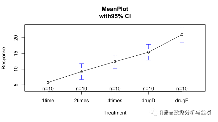
从输出结果可以知道:drugE 20.94752降低的胆固醇最多,1time 5.78197降低的胆固醇最少,各组的标准差相对恒定,在2.88-3.48之间浮动。ANOVA对治疗方式(trt)的F检验非常显著。
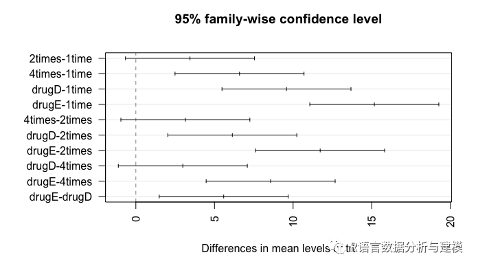
F检验表明五种药物疗法的效果不同,但是没有告诉哪种疗法与其他疗法不同。多重比较可以解决这个问题。
TukeyHSD(fit)
par(las=2)
par(mar=c(5,8,4,2))
plot(TukeyHSD(fit))
结果如下:
> TukeyHSD(fit)
Tukey multiple comparisons of means
95% family-wise confidence level
Fit: aov(formula = response ~ trt)
$trt
diff lwr upr p adj
2times-1time 3.44300 -0.6582817 7.544282 0.1380949
4times-1time 6.59281 2.4915283 10.694092 0.0003542
drugD-1time 9.57920 5.4779183 13.680482 0.0000003
drugE-1time 15.16555 11.0642683 19.266832 0.0000000
4times-2times 3.14981 -0.9514717 7.251092 0.2050382
drugD-2times 6.13620 2.0349183 10.237482 0.0009611
drugE-2times 11.72255 7.6212683 15.823832 0.0000000
drugD-4times 2.98639 -1.1148917 7.087672 0.2512446
drugE-4times 8.57274 4.4714583 12.674022 0.0000037
drugE-drugD 5.58635 1.4850683 9.687632 0.0030633
> par(las=2)
> par(mar=c(5,8,4,2))
> plot(TukeyHSD(fit))
从输出的结果可以看到1time和2times的均值差异并不明显,而1time和4times的差异非常显著。
改进一下图形:glht()函数提供多重均值比较更为全面的方法。
par(mar=c(5,4,6,2))
tuk<-glht(fit,linfct=mcp(trt="Tukey"))
plot(cld(tuk,level=0.05),col="lightgrey")
结果如下:
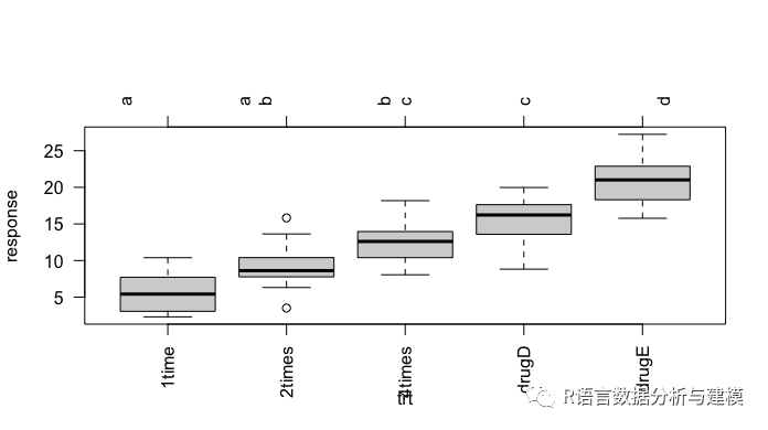
这张图的结果更加清楚明了
三.单因素协方差分析
单因素协方差分析(ANCOVA)扩展因素方差分析,包含一个或者多个定量的斜方差。
调用multcomp包中的litter数据
data(litter,package = "multcomp")
attach(litter)
table(dose)
aggregate(weight,by=list(dose),FUN=mean)
fit<-aov(weight~gesttime+dose)
summary(fit)
effect("dose",fit)
结果如下:
> table(dose)
dose
0 5 50 500
20 19 18 17 从中可以看到500的剂量,产生的数量最多
> aggregate(weight,by=list(dose),FUN=mean)
Group.1 x
1 0 32.30850
2 5 29.30842
3 50 29.86611
4 500 29.64647
> fit<-aov(weight~gesttime+dose)
> summary(fit)
Df Sum Sq Mean Sq F value Pr(>F)
gesttime 1 134.3 134.30 8.049 0.00597 **
dose 3 137.1 45.71 2.739 0.04988 *
Residuals 69 1151.3 16.69
---
Signif. codes: 0 ‘***’ 0.001 ‘**’ 0.01 ‘*’ 0.05 ‘.’ 0.1 ‘ ’ 1
> library(effects)
> effect("dose",fit)
dose effect
dose
0 5 50 500
32.35367 28.87672 30.56614 29.33460
剂量的F检验虽然表明不同的处理方式幼崽的体重均值不同,但是无法告知哪种处理方式与其他方式不同,multcomp包还可以检验用户自定义的均值假设。
评估检验的假设条件和结果可视化
library(multcomp)
fit2<-aov(weight~gesttime*dose,data=litter)
summary(fit2)
library(lattice)
library(grid)
library(latticeExtra)
library(gridExtra)
install.packages("HH")
library(HH)
ancova(weight~gesttime+dose,data=litter)
结果如下:
> library(HH)
> ancova(weight~gesttime+dose,data=litter)
Analysis of Variance Table
Response: weight
Df Sum Sq Mean Sq F value Pr(>F)
gesttime 1 134.30 134.304 8.0493 0.005971 **
dose 3 137.12 45.708 2.7394 0.049883 *
Residuals 69 1151.27 16.685
---
Signif. codes: 0 ‘***’ 0.001 ‘**’ 0.01 ‘*’ 0.05 ‘.’ 0.1 ‘ ’ 1
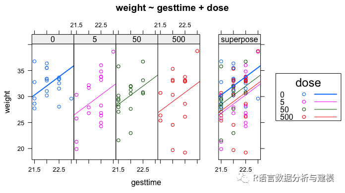
图中可以看到通过怀孕时间预测体重的线基本平行,只是截距不同,其中0剂量的截距最大,5剂量的截距最小。
四.双因素方差分析
双因素方差分析(Two-way ANOVA)有两种类型:一个是无交互作用的双因素方差分析,另一个是有交互作用的双因素方差分析,它假定因素A和因素B的结合会产生出一种新的效应。
用ToothGrowth的数据举个例子
attach(ToothGrowth)
table(supp,dose)
aggregate(len,by=list(supp,dose),FUN=mean)
dose<-factor(dose)
fit<-aov(len~sup*dose)
supp2<-supp
summary(fit)
detach(ToothGrowth)
aggregate(len,by=list(supp,dose),FUN=sd)
结果如下:
> table(supp,dose)
dose
supp 0.5 1 2
OJ 10 10 10
VC 10 10 10
> aggregate(len,by=list(supp,dose),FUN=mean)
Group.1 Group.2 x
1 OJ 0.5 13.23
2 VC 0.5 7.98
3 OJ 1 22.70
4 VC 1 16.77
5 OJ 2 26.06
6 VC 2 26.14
> dose<-factor(dose)
> fit<-aov(len~supp*dose)
> supp2<-supp
> summary(fit)
Df Sum Sq Mean Sq F value Pr(>F)
gesttime 1 134.3 134.30 8.049 0.00597 **
dose 3 137.1 45.71 2.739 0.04988 *
Residuals 69 1151.3 16.69
---
Signif. codes: 0 ‘***’ 0.001 ‘**’ 0.01 ‘*’ 0.05 ‘.’ 0.1 ‘ ’ 1
> detach(ToothGrowth)
> aggregate(len,by=list(supp,dose),FUN=sd)
Group.1 Group.2 x
1 OJ 0.5 4.459709
2 VC 0.5 2.746634
3 OJ 1 3.910953
4 VC 1 2.515309
5 OJ 2 2.655058
6 VC 2 4.797731
> attach(ToothGrowth)
The following object is masked _by_ .GlobalEnv:
dose
The following objects are masked from ToothGrowth (pos = 3):
dose, len, supp
The following objects are masked from ToothGrowth (pos = 4):
dose, len, supp
The following objects are masked from ToothGrowth (pos = 5):
dose, len, supp
The following objects are masked from ToothGrowth (pos = 6):
dose, len, supp
> table(supp,dose)
dose
supp 0.5 1 2
OJ 10 10 10
VC 10 10 10
> aggregate(len,by=list(supp,dose),FUN=mean)
Group.1 Group.2 x
1 OJ 0.5 13.23
2 VC 0.5 7.98
3 OJ 1 22.70
4 VC 1 16.77
5 OJ 2 26.06
6 VC 2 26.14
> dose<-factor(dose)
> fit<-aov(len~supp*dose)
> supp2<-supp
> summary(fit)
Df Sum Sq Mean Sq F value Pr(>F)
supp 1 205.4 205.4 15.572 0.000231 ***
dose 2 2426.4 1213.2 92.000 < 2e-16 ***
supp:dose 2 108.3 54.2 4.107 0.021860 *
Residuals 54 712.1 13.2
---
Signif. codes: 0 ‘***’ 0.001 ‘**’ 0.01 ‘*’ 0.05 ‘.’ 0.1 ‘ ’ 1
> detach(ToothGrowth)
> aggregate(len,by=list(supp,dose),FUN=sd)
Group.1 Group.2 x
1 OJ 0.5 4.459709
2 VC 0.5 2.746634
3 OJ 1 3.910953
4 VC 1 2.515309
5 OJ 2 2.655058
6 VC 2 4.797731
可视化
aggregate(len,by=list(supp,dose),FUN=sd)
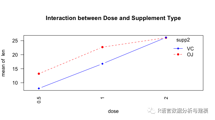
interaction.plot(dose,supp2,len,type = "b",col=c("red","blue"),pch=c(16,18),main="Interaction between Dose and Supplement Type")
library(gplots)
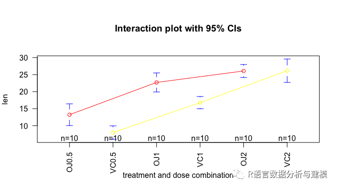
plotmeans(len~interaction(supp,dose,sep=""),connect=list(c(1,3,5),c(2,4,6)),col=c("red","yellow"),main="Interaction plot with 95% CIs",xlab="treatment and dose combination")
library(HH)
interaction2wt(len~supp*dose)
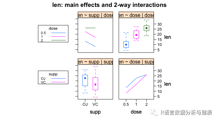
以上三幅图都表明随着橙汁和维生素c中的抗坏血酸剂量的增加,牙齿的长度变长,对于0.5和1de 剂量,橙汁比vc更能促进牙齿的增长,而对于2ml的剂量,两者的增长速度相同。
四.重复测量的方差分析
重复测量方差分析是指被试者的测量不止一次。
CO2$conc<-factor(CO2$conc)
w1b1<-subset(CO2,Treatment=="childed")
fit<-aov(uptake~conc*Type+Error(Plant/(conc)),w1b1)
summary(fit)
结果如下:
summary(fit)
Df Sum Sq Mean Sq F value Pr(>F)
supp 1 205.4 205.4 15.572 0.000231 ***
dose 2 2426.4 1213.2 92.000 < 2e-16 ***
supp:dose 2 108.3 54.2 4.107 0.021860 *
Residuals 54 712.1 13.2
---
Signif. codes: 0 ‘***’ 0.001 ‘**’ 0.01 ‘*’ 0.05 ‘.’ 0.1 ‘ ’ 1
五.多元方差分析
我们采用uscereal 中的数据来研究食物中的卡路里,脂肪,糖类是否会随着存储位置的不同而发生变化
library(MASS)
attach(UScereal)
shelf<-factor(shelf)
y<-cbind(calories,fat,sugars)
aggregate(y,by=list(shelf),FUN=mean)
summary(fit)
结果如下:
shelf<-factor(shelf)
> y<-cbind(calories,fat,sugars)
> aggregate(y,by=list(shelf),FUN=mean)
Group.1 calories fat sugars
1 1 119.4774 0.6621338 6.295493
2 2 129.8162 1.3413488 12.507670
3 3 180.1466 1.9449071 10.856821
> summary(fit)
Df Sum Sq Mean Sq F value Pr(>F)
supp 1 205.4 205.4 15.572 0.000231 ***
dose 2 2426.4 1213.2 92.000 < 2e-16 ***
supp:dose 2 108.3 54.2 4.107 0.021860 *
Residuals 54 712.1 13.2
---
Signif. codes: 0 ‘***’ 0.001 ‘**’ 0.01 ‘*’ 0.05 ‘.’ 0.1 ‘ ’ 1
