


two-phase sampling
两相采样
8.1 multistage and multiphase sampling
8.1 多级和多相采样
Multistage sampling, as described in Chapter 3, requires the assumption that the subsampling of one PSU does not depend on which other PSUs were sampled.
如第 3 章所述,多阶段抽样要求假设一个初级抽样单位的子抽样不取决于对哪些其他初级抽样单位进行抽样。
It is possible to relax this assumption and to allow subsampling that depends on all the currently observed data at each step, a process called multiphase sampling.
可以放宽这个假设,并允许在每个步骤依赖于所有当前观察到的数据进行二次采样,这个过程称为多相采样。
This chapter discusses two scenarios where two-phase sampling is helpful in designing subsamples.
本章讨论两阶段采样有助于设计子样本的两种情况。
There are many other possible two-phase and multiphase sampling designs, including longitudinal designs where overlapping samples are taken on multiple occasions, and dual-frame designs where samples are taken from two incomplete population lists.
还有许多其他可能的两阶段和多阶段采样设计,包括在多次重叠样本的纵向设计,以及从两个不完整的总体列表中抽取样本的双帧设计。
At the time of writing these other designs are not directly supported in the survey package, although it should be possible to translate instructions for analyzing them using other software into R.
在撰写本文时,survey包不直接支持这些其他设计,尽管应该可以将使用其他软件分析它们的指令翻译成 R。
The distinction between two-stage and two-phase subsampling is important theoretically, although it has relatively little impact on applied analysis of subsampling designs.
两阶段和两阶段子采样之间的区别在理论上很重要,尽管它对子采样设计的应用分析影响相对较小。
The reason for the theoretical distinction is that it is not possible to calculate the true sampling probability for an individual.
理论上存在差异的原因是无法计算个体的真实抽样概率。
We have available the probability ni(1) that individual i is in the first-phase sample, and the probability ni(q1) that that the individual is then included at phase two.
我们有可用的概率的Ni(1) ,个别我是第一阶段的样品中,和概率NI(Q1)的是其的个体,然后在包含第二阶段。
For multistage sampling, in Chapter 3 we could simply multiply the stage-one and stage-two probabilities to obtain ni , because of the assumption that subsampling for one cluster did not depend on anything outside that cluster.
对于多阶段采样,在第3章中,我们可以简单地将第一阶段和第二阶段的概率相乘以获得ni ,因为假设一个集群的子采样不依赖于该集群之外的任何东西。
The purpose of two-phase designs is to relax this assumption so the subsampling probability can be based on the composition of the first-phase sample and could be different for other first-phase samples.
两阶段设计的目的是放宽这一假设,因此子采样概率可以基于第一阶段样本的组成,并且对于其他第一阶段样本可能不同。
In order to compute the probability that individual i is in the sample we would need to average ni(1) x ni(211) over all possible first-phase samples that include individual i , which typically requires data we do not have as well as being computationally infeasible.
为了计算个体i在样本中的概率,我们需要对包含个体i 的所有可能的第一阶段样本求平均ni(1) x ni(211) ,这通常需要我们没有的数据以及在计算上不可行。
Fortunately, the numbers nr = ni(1) x ni(2ll) can be used in the same way as ni to create sampling weights that give unbiased estimators of the population total, and the corresponding pairwise numbers can be used to estimate standard errors.
幸运的是,数字nr = ni(1) x ni(2ll)可以以与ni相同的方式用于创建抽样权重,从而给出总体总数的无偏估计量,并且相应的成对数字可用于估计标准误差。
The resulting estimator is not the Horvitz-Thompson estimator, but it looks, walks, and quacks like it.
所得到的估计是不是霍维茨-Thompson估计,但看起来,散步,和叫声也像它。
The mathematical details of estimation are given in Chapter 9 of S h d a l et al [151], much of which follows S h d a l and Swensson [150].
估计的数学细节在 S hdal 等人 [151] 的第 9 章中给出,其中大部分遵循 S hdal 和 Swensson [150]。
Two-phase samples can be described to R with the function twophase().
两相的样品可以用功能进行描述R的twophase() 。
At the time of writing the designs that can be handled are relatively restricted.
在撰写本文时,可以处理的设计相对有限。
Either phase one is a stratified sample of individuals, or phase one is a cluster sample in which all clusters are represented at phase two.
第一阶段是个人分层样本,或者第一阶段是集群样本,其中所有集群都在第二阶段表示。
The call to twophase() has similar arguments to the call to mydesign( 1, but each argument is a list of two formulas rather than a single formula, representing the two phases of sampling.
调用twophase()具有类似于参数调用mydesign(1,但是每个参数是两个公式,而不是一个单一的式,代表取样的两个阶段的列表。
More detail is given in the examples in section 8.4
更多细节在第8.4节的示例中给出
8.2 sampling for stratification
8.2 分层抽样
Two-phase sampling for stratification can be used when a valuable stratification variable is not available for all individuals in the population but can be measured inexpensively.
当有价值的分层变量不适用于总体中的所有个体但可以廉价测量时,可以使用用于分层的两阶段抽样。
The strategy is to take a large sample from the population, measure the stratification variable, and then take a stratified subsample.
策略是从总体中抽取一个大样本,测量分层变量,然后再抽取一个分层的子样本。
The phase-one sample can be a simple random sample or can be stratified on other variables that are available for the population.
第一阶段样本可以是简单的随机样本,也可以根据总体可用的其他变量进行分层。
If the phase-one sample is sufficiently large, the distribution of the stratifying variable across the phase-one sample will be very similar to the distribution across the population, and the design will give very similar estimates to the stratified one-phase design it is emulating (Exercise 8.1).
如果第一阶段样本足够大,第一阶段样本中分层变量的分布将与总体分布非常相似,并且设计将给出与分层一阶段设计非常相似的估计值模拟(练习 8.1)。
One situation where two-phase sampling for stratification has been popular is in estimating the age distribution of fish caught by the commercial fishing industry.
用于分层的两阶段抽样流行的一种情况是估计商业捕鱼业捕获的鱼的年龄分布。
Kutkuhn [88] describes a two-phase sampling system for the California salmon catch, where fish size is measured on a large sample of fish at the port and then used to choose a stratified subsample of fish to have age determined accurately by counting rings on scales.
Kutkuhn [88]描述了加利福尼亚鲑鱼捕捞的两阶段采样系统,在该系统中,在港口的大量鱼样本上测量鱼的大小,然后用于选择分层的鱼子样本,通过计数环来准确确定鱼的年龄。秤。
Smith [164] describes a similar system for estimating the age distribution of halibut, and concludes that the phase-one sampling is sufficiently expensive that a simple random sample would be more cost-effective.
Smith [164] 描述了一种用于估计大比目鱼年龄分布的类似系统,并得出结论,第一阶段采样的成本足够高,因此简单的随机样本更具成本效益。
Screening of a phase-one sample for stratification in psychiatric research is described by Pickles et al [126].
Pickles 等人 [126] 描述了筛选用于精神学研究分层的第一阶段样本。
A simple questionnaire is administered at phase one, and the results are used to draw a stratified subsample with high sampling probabilities where the screening questionnaire indicated a high chance of mental illness.
在第一阶段管理一个简单的问卷,结果用于抽取具有高抽样概率的分层子样本,其中筛选问卷表明精神疾病的可能性很高。
NHANES and NHIS use a screening design based on ethnicity in the third and fourth stage of their multistage sample (Mohadjer and Curtin[l09]).
NHANES 和 NHIS 在其多阶段样本的第三和第四阶段使用基于种族的筛选设计(Mohadjer 和 Curtin [109])。
After small clusters of households have been chosen in a two-stage design, some household clusters are screened and included in the sample only if they include one or more black, Asian, or Hispanic persons.
在两阶段设计中选择小家庭集群后,一些家庭集群仅在包含一名或多名黑人、亚洲人或西班牙裔人的情况下才被筛选并纳入样本。
This two-phase sampling is not represented in the public-use data files and so cannot be incorporated in any secondary analysis.
该二相采样未在公共使用的数据文件表示,所以不能在任何二次分析并入。
I do not know if the internal analyses at the National Center for Health Statistics explicitly incorporate the two-phase structure of the sample.
我不知道,如果在全国卫生统计中心的内部分析明确地纳入样本的两相结构。
8.3 THE CASE-CONTROL DESIGN
8.3病例 - 对照设计
Probably the most important example of sampling for stratification is the classical case-control design (or choice-based design in economics).
分层抽样最重要的例子可能是经典的病例对照设计(或经济学中的基于选择的设计)。
The case-control design is used in epidemiology to study rare diseases such as cancers, where any of the sampling designs we have seen so far would end up sampling very few people with the disease.
病例对照设计在流行病学中用于研究癌症等罕见疾病,到目前为止我们所看到的任何抽样设计最终都会对极少数患有该疾病的人进行抽样。
The case-control design assumes that it is relatively easy to identify all the cases of the disease in some group of people and, implicitly, to identify all the controls, ie, people without the disease.
病例对照设计假设在某些人群中识别所有疾病病例相对容易,并且隐含地识别所有对照,即没有疾病的人。
The first phase of sampling results in the group of people whose disease status is known.
其疾病状态是已知的,一群人在抽检结果的第一阶段。
In the second phase all the cases are sampled, but only a small fraction of the controls - typically 1-5 times as many controls as cases.
在第二阶段,所有案例都被采样,但只有一小部分控制——通常是案例数量的 1-5 倍。
Predictor variables are then measured on the second-phase sample.
预测变量然后在第二阶段的样品进行测定。
If the cases make up 1/1000 of the population and the same number of cases as controls is used, the sampling fractions will be 1 for cases and 1/1000 for controls.
如果病例占总体的 1/1000,并且使用的病例数与对照相同,则采样分数将是病例的 1 和对照的 1/1000。
The design effect for a case-control sample is of the same order of magnitude as the sampling probability for controls; the design is enormously more efficient than simple random sampling.
病例对照样本的设计效果与对照的抽样概率处于同一数量级;这种设计比简单的随机抽样更有效。
When the cases come from a well-defined population and the controls genuinely are a random sample of the same population, the design is called population-based.
当案例来自定义明确的总体并且对照确实是同一总体的随机样本时,该设计称为基于总体的设计。
For example, the cases may be all the stroke cases at a particular HMO and the controls a sample from HMO members, or the cases may be all the cancer cases in a particular state and the controls a sample from the population of that state.
例如,病例可能是特定 HMO 的所有中风病例和来自 HMO 成员的样本,或者病例可能是特定州的所有癌症病例和来自该州人口的样本。
It is often hard to establish a population for the cases, and so controls are often sampled in ways that only approximate the formal case-control design - not surprisingly, problems with the choice of controls are a common criticism of these designs.
通常很难为案例建立总体,因此控制通常以仅近似于正式案例控制设计的方式进行抽样-毫不奇怪,控制选择的问题是对这些设计的普遍批评。
A historical review of the case-control design is given by Breslow [12].
Breslow [ 12]对病例对照设计进行了历史回顾。
In fact it is unusual for design-based inference to be used in the case-control design.
事实上,在案例控制设计中使用基于设计的推理是不寻常的。
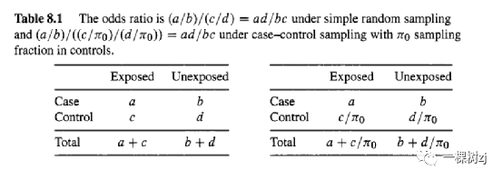
The usual analysis relies on the fact that one particular association measure, the odds ratio, can be estimated correctly without using sampling weights as long as the logistic regression model is correctly specified.
通常的分析依赖于这样一个事实:只要正确指定逻辑回归模型,就可以在不使用采样权重的情况下正确估计一个特定的关联度量,即优势比。
With a single binary predictor variable this result is elementary (Table 8.1): the odds of exposure in cases does not depend on the controls in any way, and the odds of exposure in controls does not depend on the sampling fraction for controls because all controls have the same sampling probability.
对于单个二元预测变量,此结果是基本的(表 8.1):病例中的暴露几率不以任何方式取决于对照,并且对照中的暴露几率不取决于对照的抽样比例,因为所有对照具有相同的抽样概率。
The general result for discrete variables was given by Anderson [ l ] and for continuous variables by Prentice and Pyke [ 1281.
Anderson [l] 给出了离散变量的一般结果,Prentice 和 Pyke [ 1281 ] 给出了连续变量的一般结果。
In addition to simplicity of estimation and the fact that it can be applied without knowing the population sizes, the unweighted estimator always has the same or smaller standard errors.
除了估计的简单性以及它可以在不知道总体规模的情况下应用的事实之外,未加权的估计量始终具有相同或较小的标准误差。
In some situations the gain in precision can be quite large, for example, Scott and Wild [158] showed simulations where the weighted estimator would need up to eight times the sample size to obtain the same precision.
在某些情况下在精密的增益可以是相当大的,例如,Scott和野生[158]显示模拟,其中所述加权估计将需要多达八个倍样品量以获得相同的精度。
On the other hand, the difference in precision is small when the odds ratio is not far from 1, and simulations using different distributions from those used by Scott and Wild show smaller differences in precision even at large odds ratios.
另一方面,当优势比不远为 1 时,精度差异很小,并且使用与 Scott 和 Wild 使用的分布不同的分布的模拟显示,即使在优势比很大的情况下,精度差异也较小。
Some of these simulations are presented in section 8.3.1.
其中一些模拟的第8.3.1节介绍。
The disadvantage of the unweighted estimator is the fact that its validity relies on the logistic regression model being correct, something that many statisticians are reluctant to assume.
未加权估计量的缺点是其有效性依赖于逻辑回归模型的正确性,这是许多统计学家不愿假设的。
As Scott and Wild[158] observe The usual practice when building parametric regression models is to start with simple candidate surfaces and to complicate them only when the data force us to do so.
正如Scott 和 Wild [158] 所观察到的,构建参数回归模型的通常做法是从简单的候选曲面开始,只有在数据迫使我们这样做时才将它们复杂化。
As a consequence, we are always working with a model that is not quite right.
作为结果,我们总是与一个模型,是不完全正确的工作。
We saw in Chapter 5 that the weighted estimator always estimates a well-defined quantity, the best-fitting population logistic model, even if the model is not exactly correct.
我们在第5章中看到,加权估计量总是估计一个明确定义的数量,即最适合的总体逻辑模型,即使该模型不完全正确。
The potential for being misled by bias is less serious than in the scenarios in Chapter 5.
被偏见误导的可能性没有第5章中的情景严重。
Using the weights gives the best-fitting logistic regression model in the population, omitting the weights gives the best-fitting regression model in a modified population where the risk of disease is higher at any covariate value [158].
使用权重给出了人群中最合适的逻辑回归模型,省略权重给出了修改后的人群中最合适的回归模型,其中任何协变量值的疾病风险都较高 [158]。
In the past this issue has been quite controversial in statistics.
在对过去这个问题一直在统计颇有争议。
It now seems that both the bias from a misspecified model and the precision gain from avoiding weights are smaller than they were feared to be.
现在看来,错误指定模型的偏差和避免权重带来的精度增益都比他们担心的要小。
For the relative small effect sizes that are most common it appears that there is no compelling argument in either direction and a reasonable approach might be to fit both the weighted and unweighted estimators.
对于相对小的影响的大小是最常见的,似乎有沿任一方向没有令人信服的理由和合理的方法可能是适合的加权和非加权估计两者。
Example: Oesophageal cancer in Me-ef-Vilaine.
示例:Me-ef-Vilaine 的食道癌。
Breslow and Day[ 141 used as an example a case-control study of oesophageal cancer conducted in the Ille-et- Vilaine region of northwest France by Tuyns et al [176].
布瑞斯罗夫和日[141用作一个例子由Tuyns等人[176]在法国西北部的伊勒- ET-维莱讷区域进行食道癌的病例-对照研究。
The control sampling probability for these data was not reported by Tuyns et al. [176], but in an earlier paper [175] reporting cancer incidence rates they gave the population of the dkpurtement of Ille-et-Vilaine as 430,000, implying a control sampling probability of 0.00225, or a sampling weight of 441.
Tuyns 等人没有报告这些数据的控制抽样概率。[176],但在较早的一篇报告癌症发病率的论文 [175] 中,他们给出了Ille-et-Vilaine的dkpurtement人口为 430,000,这意味着控制抽样概率为 0.00225,或抽样权重为 441。
As the phase one sample is large, treating the design as a single phase of stratified sampling with replacement gives an essentially identical answer to using the full two-phase representation, so it is not necessary to construct a data set with the 429,000 controls in Ille-et-Vilaine who were implicitly in the phase-one sample.
由于第一阶段样本很大,将设计视为带有替换的分层抽样的单阶段给出了与使用完整两阶段表示基本相同的答案,因此没有必要使用 Ille 中的 429,000 个对照构建数据集-et-Vilaine 隐含在第一阶段样本中。
Exercise 8.2 does construct the full two-phase representation to confirm that the same result is obtained.
练习 8.2 确实构造了完整的两阶段表示以确认获得了相同的结果。
The data are built in to R, in a data set called esoph, but in a tabular form listing the number of cases and controls for 88 combinations of predictors.
数据内置于 R 中,位于名为esoph的数据集中,但以表格形式列出了88种预测变量组合的病例数和对照。
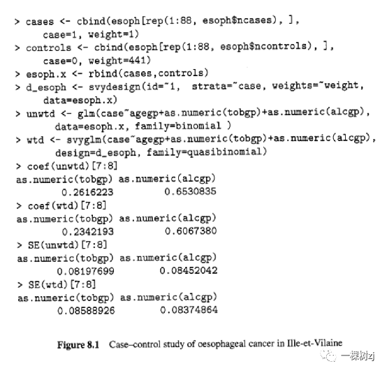
The code in Figure 8.1 expands the data to one record for each person and creates the weight variable, then performs weighted and unweighted logistic regressions.
图 8.1 中的代码将数据扩展为每个人的一条记录并创建权重变量,然后执行加权和未加权的逻辑回归。
The model, which fits the data well, has linear terms in the grouped tobacco and alcohol variables and a separate indicator variable for each age group.
该模型很好地拟合了数据,在分组的烟草和酒精变量中具有线性项,并且每个年龄组都有一个单独的指标变量。
The estimated log odds ratios are very similar in the two models, and highly statistically significant.
两个模型中估计的对数优势比非常相似,并且具有高度的统计显着性。
The standard errors from the unweighted model are 5% smaller for the tobacco coefficient and essentially identical for the alcohol coefficient.
来自未加权模型的标准误差对于烟草系数小5% ,对于酒精系数基本上相同。
In this example there is little inefficiency from using the weights, but also little difference in the estimates, and the same inference would be drawn from either analysis.
在这个例子中,使用权重几乎没有效率低下,但估计值也几乎没有差异,并且可以从任一分析中得出相同的推论。
8.3.1 * Simulations: efficiency of the design-based estimator
8.3.1 *模拟:基于设计估计的效率
There are two approaches to simulating a case-control design.
有两种方法来模拟病例 - 对照设计。
The simplest is to simulate the phase-one sample and subsample from it.
最简单的方法是模拟第一阶段样本及其子样本。
This tends to be slow, especially on computers with limited memory, when the sampling fraction for controls is small.
这往往很慢,特别是在内存有限的计算机上,当控件的采样分数很小时。
For example, simulating the Ille-et-Vilaine case-control design would require repeatedly simulating a population of size 430,000.
例如,模拟 Ille-et-Vilaine 病例控制设计将需要重复模拟 430,000 人口。
The other approach is to specify the covariate distribution in controls and then use the relationship
另一种方法是指定在控制协变量的分布,然后使用关系
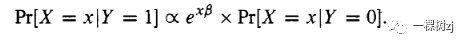
For discrete covariates this exponential tilting procedure gives the case distribution directly.
对于离散协变量,这种指数倾斜程序直接给出案例分布。
For continuous covariates from an exponential family distribution, in particular the Normal distribution, it is also straightforward to compute the distribution in cases.
对于来自指数族分布的连续协变量,特别是正态分布,计算个案中的分布也很简单。
The second approach is less general, since it can be used only when the true relationship is logistic and when the predictor distribution in controls makes exponential tilting easy, and it is difficult to adapt to complex sampling at phase one.
第二种方法不太通用,因为它只能在真实关系是逻辑关系并且控制中的预测变量分布使指数倾斜容易时使用,并且难以适应第一阶段的复杂采样。
When examining the efficiency of the weighted estimator the extra generality provided by simulating the entire first-phase sample is not necessary.
在检查加权估计器的效率时,不需要通过模拟整个第一阶段样本提供的额外通用性。
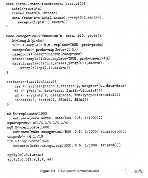
The code in Figure 8.2 creates Normal or categorical data and fits the logistic regression model using both the weighted and unweighted estimators.
图 8.2 中的代码创建正常或分类数据,并使用加权和未加权估计量拟合逻辑回归模型。
It then performs 1000 replications of a simulation with /I = 0.5, 500 cases and 500 controls, and a control sampling fraction of 1/1000, for three data distributions.
然后,对于三个数据分布,它使用/I = 0.5、500 个案例和 500 个控制以及 1/1000 的控制抽样比例执行模拟的 1000 次复制。
The first is a Normal distribution, the second is a square distribution taking values 1 4 with equal probability in controls, and the third is a triangular distribution taking values 1 4 with probabilities 0.4,0.3, 0.2,0.l in controls.
第一个是正态分布,第二个是正方形分布,在控件中取值 1 4 的概率相等,第三个是三角形分布,在控件中取值 1 4 ,概率为0.4,0.3, 0.2,0.l。
The calls to apply() compute the means and standard errors of the estimators.
对apply()的调用计算估计量的均值和标准误差。
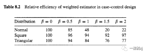
Table 8.2 shows the results of running these three simulations and repeating them for B = 0,0.5,1,1.5,2.
表 8.2 显示了运行这三个模拟并针对B = 0、0.5、1、1.5、2重复它们的结果。
The number in each cell of the table is the relative efficiency of the weighted estimator.
表中每个单元格中的数字是加权估计量的相对效率。
If the relative efficiency is 50%, the weighted estimator requires twice as many observations for the same accuracy.
如果相对效率为50%,则加权估计量需要两倍于相同精度的观测值。
The results for the Normal distribution agree with those of Scott and Wild [158], but the results for the two discrete distributions show much less difference between the two estimators.
正态分布的结果与 Scott 和 Wild [158]的结果一致,但两个离散分布的结果显示两个估计量之间的差异要小得多。
The distribution of alcohol and tobacco intake for the Ille-et-Vilaine oesophageal cancer study is similar to the triangular distribution in the simulations.
Ille-et-Vilaine 食管癌研究的酒精和烟草摄入量分布类似于模拟中的三角形分布。
The efficiency of the weighted estimator is slightly higher for the Ille-et-Villaine data set than in the simulations because there are approximately five times as many controls as cases.
Ille-et-Villaine 数据集的加权估计器的效率比模拟中的略高,因为控制的数量大约是案例数量的五倍。
8.3.2 Frequency matching
8.3.2 频率匹配
Many case-control designs use a further level of stratification and unequal sampling in the phase-two sample, a practice known in the epidemiology literature as frequency matching.
许多病例对照设计在第二阶段样本中使用更深层次的分层和不等抽样,这在流行病学文献中称为频率匹配。
The goal of frequency matching is to prevent small case vs control differences in the exposure under study from being masked by very large differences in another variable whose effects are known and not of interest.
频率匹配的目标是防止所研究的暴露中的小病例与对照差异被另一个变量的非常大的差异所掩盖,该变量的影响是已知的而不是感兴趣的。
For example, in the oesphageal cancer study described above, very little information about the effects of alcohol and tobacco is present in the youngest age group, because there is only one case.
例如,在上述食管癌研究中,关于酒精和烟草影响的信息很少出现在最年轻的年龄组中,因为只有一个案例。
If the associations with age had already been understood and the study had been designed to estimate the effect of alcohol and tobacco this would be an inefficient design that effectively wasted 116 controls.
如果随着年龄的关联已经了解和学习了旨在估算酒精和烟草的影响,这将是一个低效率的设计,有效地浪费116所控制。
A more efficient design would sample more controls at older ages and end up with five controls per case in each age group rather than five controls per case on average over all ages.
一个更有效的设计会在老年阶段品尝更多的控制,并与各年龄组的情况下,每五个控件,而不是在所有年龄段每箱五个控件平均告终。
Frequency matching is not the most efficient way to use the age information in a two-phase design, but it has the advantage that an unweighted analysis is still valid as long as the stratification variables are included in the model.
频率匹配不是在两阶段设计中使用年龄信息的最有效方法,但它的优点是只要模型中包含分层变量,未加权分析仍然有效。
The coefficients for the stratification variables will not be correct, but these are assumed to be uninteresting.
对于分层变量的系数将是不正确的,但这些被假定为无趣。
The coefficients for other variables will be correct under the same assumption of a correct model that was made for a unmatched case-control design.
在为不匹配的病例对照设计制作的正确模型的相同假设下,其他变量的系数将是正确的。
8.4 sampling from existing cohorts
8.4从现有队列中抽样
In two-phase sampling for stratification there is very little information available at phase one, and most variables are measured only at phase two.
在用于分层的两阶段抽样中,第一阶段可用的信息很少,大多数变量仅在第二阶段进行测量。
The opposite situation is rare in official statistics but occurs in epidemiologic studies when new variables are measured on a subset of an existing sample; many variables at phase one and only a little extra information at phase two.
相反的情况在官方统计中很少见,但在流行病学研究中发生,当对现有样本的一个子集测量新变量时;第一阶段有很多变量,第二阶段只有很少的额外信息。
Large observational cohort studies and randomized trials recruit a sample of thousands of people (treated for analysis purposes as a simple random sample from a very large population) and measure hundreds of variables over years or decades of follow-up.
大型观察性队列研究和随机试验招募了数千人的样本(出于分析目的,将其视为来自大量人口的简单随机样本),并在数年或数十年的随访中测量数百个变量。
As new research questions and measurement techniques arise, investigators need to measure new variables.
随着新的研究问题和测量技术的出现,研究人员需要测量新的变量。
These may be new assays of stored blood and DNA samples, data from reviews of medical records, or simply coding and entry of free-text questions on, eg, nutritional supplements or over-the-counter medications.
这些可能是对存储的血液和 DNA 样本的新分析、来自医疗记录审查的数据,或者简单地编码和输入关于例如营养补充剂或非处方药的自由文本问题。
Measuring these new variables is often expensive, so restricting the new measurements to a subsample of the full cohort is desirable.
测量这些新变量通常很昂贵,因此将新测量限制在整个队列的子样本中是可取的。
Rather than taking a simple random sample, it is more efficient to use the existing variables to stratify the sampling.
与采用简单的随机样本相比,使用现有变量对抽样进行分层更有效。
The traditional approach was to stratify on a single outcome variable, giving a nested case-control or case-cohort [ 1271 design.
传统的方法是对单个结果变量进行分层,给出嵌套的病例对照或病例队列[ 1271 设计。
Data from phase one for individuals not in the phase-two sample was ignored.
不属于第二阶段样本的个体的第一阶段数据被忽略。
More recently, epidemiologists have become aware of the potential advantages of stratifying the phase-two sample on predictors as well as response, and of poststratifying or calibrating the phase-two sample to the full cohort.
最近,流行病学家已经意识到根据预测因子和响应对第二阶段样本进行分层以及将第二阶段样本后分层或校准到完整队列的潜在优势。
As with the nested case-control design there are sampling-weighted estimators that do not rely on the assumption that a model has been correctly specified, and semiparametric maximum likelihood estimators that do make this assumption.
与嵌套病例对照设计一样,存在不依赖于模型已正确指定的假设的抽样加权估计量,以及做出此假设的半参数最大似然估计量。
The relative importance of the bias from assuming the model is correct and the efficiency loss from not assuming it is correct are even less well understood than in the nested case-control design, and two-phase model-based estimation is an area of active research at the time of writing.
假设模型正确的偏差的相对重要性和不正确假设的效率损失比嵌套病例控制设计更难理解,基于两阶段模型的估计是一个活跃的研究领域在撰写本文时。
8.4.1 Logistic regression
8.4.1逻辑回归
In the 2 x 2 table in Table 8.1 the estimated variance of the log odds ratio is
在表 8.1的 2 x 2 表中,对数优势比的估计方差为
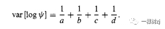
The case-control design ensures that the number of cases, a + b , and the number of controls, c + d , are both large, but if exposure is rare it is still possible for a or c to be small.
病例对照设计确保病例数a + b和对照数c + d都很大,但如果曝光很少,a或c仍然可能很小。
For example, consider the data in Table 8.3, from the National Wilms Tumor Study Group [54, 381.
例如,请考虑来自 National Wilms Tumor Study Group [54, 381.] 的表 8.3 中的数据。
All the participants in these studies have Wilms’ tumor, so the ‘cases’ and ‘controls’ are cases of relapse and controls who did not experience relapse.
这些研究的所有参与者都患有威尔姆斯瘤,因此“病例”和“对照”是复发病例和未复发的对照。
A case-control sample of all 669 cases and 669 of the controls from this population would, on average, include only 50 controls with unfavorable histology.
所有 669 例病例和来自该人群的 669 例对照的病例对照样本平均仅包括 50 例具有不利组织学的对照。
If sampling could be based on both exposure and outcome it would be possible to have 100% sampling of the three smaller cells, plus 424 controls with good histology, adding up to the same sample size of 669 x 2 = 1338.
如果采样可以基于曝光和结果将可能具有三个较小的细胞的100%采样,加上具有良好的组织学424所控制,加起来的669相同的样本大小X 2 = 1338。
Increasing the smallest cell count from 50 to 194 will clearly give better estimates of association.
将最小细胞数从 50 增加到 194 显然可以更好地估计关联。
Of course, sampling stratified on the cells in Table 8.3 would require knowing histologic classification and relapse status for everyone in the population and sampling would then be unnecessary.
当然,抽样分层上的表8.3的细胞需要知道每个人都在人口学分类和复发状态和采样然后是不必要的。
The question this example raises is whether the potential gains from sampling based on exposure and outcome are ever available in practice.
这个例子提出的问题是,基于暴露和结果的抽样的潜在收益是否在实践中可用。
There are at least two situations where the increased precision can be realized in practical designs.
至少有两种情况可以在实际设计中实现提高的精度。
The first is when exposure and outcome are available for all of a phase-one sample and subsampling is being used to measure additional variables that may confound or interact with the exposure.
第一种是当曝光和结果可用于所有相位一个样本的子采样和被用于测量可与曝光混淆或相互作用的附加变量。
The second is when the true exposure is not available at phase one but there are variables available that predict the outcome reasonably well.
第二种情况是在第一阶段无法获得真正的暴露,但有可用的变量可以合理地预测结果。
The Wilms’ tumor population data have been widely used as an artificial example of sampling based on a surrogate for exposure; the accounts here are based on Breslow and Chatterjee [13] and Kulich and Lin [85].
Wilms 的肿瘤种群数据已被广泛用作基于暴露替代物采样的人工示例;这里的叙述基于 Breslow 和 Chatterjee [13] 以及 Kulich 和 Lin [85]。
The histologic classification in Table 8.3 is performed at the central laboratory of the National Wilms Tumor Study Group, by the pathologist who first characterized the histologic variations of Wilms’ tumor.
表8.3中的组织学分类是在国家肾母细胞肿瘤研究组的中心实验室由病理学家谁第一特征的肾母细胞瘤组织学变化进行。
There is also available a classification by pathologists at the hospital where treatment was performed.
也有通过在那里进行治疗医院病理学家可用的分类。
These pathologists will be less familiar with Wilms’ tumor, which is a very rare disease, and their ratings might well be less accurate.
这些病理学家对维尔姆斯肿瘤不太熟悉,这是一种非常罕见的疾病,他们的评级可能不太准确。
Analyzing the complete data confirms this possibility.
分析完整数据证实了这种可能性。
The central lab classification predicts relapse rate more strongly than the local hospital classification, and if the central lab classification is known there is little or no improvement in prediction of relapse by using the local hospital classification in addition.
中心实验室分类预测复发率强于当地医院的分类,如果中心实验室的分类被称为有很少或通过另外使用本地医院分级复发的预测没有任何改善。
That is, essentially all the differences between the two sets of histologic classifications are errors by the local hospital pathologists, who have about 98% specificiLy but only about 75% sensitivity in detecting the unfavorable histology.
也就是说,基本上两组组织学分类之间的所有差异都是当地医院病理学家的错误,他们在检测不利的组织学方面具有约98%的特异性但只有约75%的敏感性。
If it became desirable to restrict the central lab evaluation to retrospective classification of a subsample of tumors, an obvious set of strata would be the four cells formed by tabulating relapse and local hospital histology.
如果希望将中央实验室评估限制为对肿瘤子样本进行回顾性分类,那么一组明显的分层将是通过将复发和当地医院组织学制成表格而形成的四个细胞。
Sampling everyone with unfavorable (local hospital) histology, all the relapse cases with favorable histology, and 449 controls with favorable (local hospital) histology, gives the same sample size of 1138 as a 1:l case-control sample.
对组织学不良(当地医院)的每个人、所有组织学良好的复发病例和 449 名组织学良好的对照(当地医院)进行抽样,得出与 1:1 病例对照样本相同的样本量 1138。
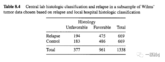
Table 8.4 shows the expected table of (central lab) histology by relapse.
表 8.4 显示了预期复发的(中心实验室)组织学表。
The smallest cell is controls with unfavorable histology, as for the case-contrd sample, but the expected number is 183 rather than 50.
对于病例对照样本,最小的细胞是组织学不良的对照,但预期数量是 183 而不是 50。
The price for the increased flexibility in sampling is that ordinary logistic regression no longer gives a valid analysis: the unweighted odds ratio in Table 8.4 is 1.08 and the true population odds ratio from Table 8.3 is 5.0.
增加抽样灵活性的代价是普通逻辑回归不再提供有效分析:表 8.4 中的未加权优势比为 1.08,而表 8.3 中的真实总体优势比为 5.0。
It is straightforward to estimate the odds ratio using weights based on nl: the subsampling probabilities ni(41) are known and since the complete sample is being modeled as a simple random sample from an infinite superpopulation all ni(1) are equal and can be taken as = 1.
使用基于nl 的权重来估计优势比很简单:子采样概率ni(41)是已知的,并且由于完整样本被建模为来自无限超总体的简单随机样本,因此所有ni(1)都是相等的,并且可以是取为= 1。
The weighted analysis also has the advantage of being able to estimate statistics other than odds ratios, such as the relative risk of relapse with poor histology or the sensitivity and specificity of the local hospital histology classification.
加权分析还具有能够估计比值比以外的统计数据的优势,例如组织学较差的复发的相对风险或当地医院组织学分类的敏感性和特异性。
Exercise 8.4 shows by simulation that the true sampling probabilities nj, which depend on the superpopulation model, are likely to be very close to n,? for this design.
通过模拟演练8.4所示,真正的抽样概率NJ,这取决于超总体模型,可能是非常接近ň,?对于这样的设计。
8.4.2 Two-phase case-control designs in R A
8.4.2 R A 中的两相工控设计
two-phase design is specified with the twophase () function.
两阶段设计是用 twophase ()函数指定的。
The syntax is similar to that for svydesign() , except that two sets of information are required, one for each phase.
语法类似于 svydesign() ,不同之处在于需要两组信息,每个阶段一组。
The i d and strata arguments are lists of two model formulas, the first for phase one, the second for phase two.
该ID和地层参数是两个模型公式列表,第一个阶段为一个,第二个为第二阶段。
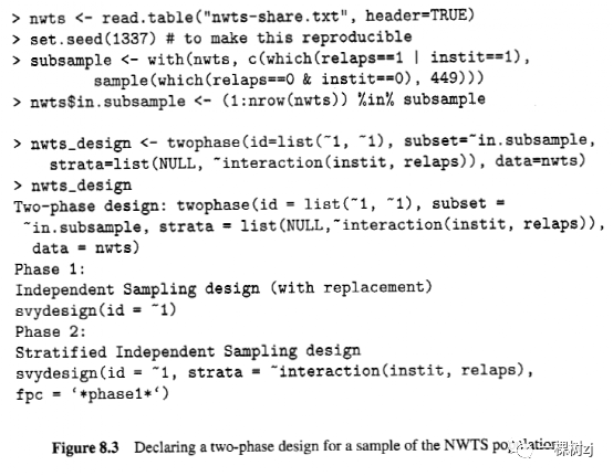
In Figure 8.3 the i d argument specifies sampling of individuals at each phase.
在图 8.3 中,id参数指定每个阶段的个体抽样。
The strata argument specifies that the first stage is unstratified and the second stage is stratified on the cross-classification of instit and relaps .
该地层参数指定第一阶段是不分层和第二级分层上instit和relaps的交叉分类。
The subset argument is a logical (TRUWFALSE) vector indicating which individuals are in phase two.
所述子集的参数是指示哪些个体在第二阶段的逻辑(TRUWFALSE)载体。
The data are supplied as a data frame with a record for every individual, whether or not they are in phase two.
数据作为数据帧提供,每个人都有记录,无论他们是否处于第二阶段。
If they are not in the phase two sample they would usually have NA values for any phasetwo variables.
如果它们不在第二阶段样本中,则它们通常具有任何第二阶段变量的NA值。
A single set of sampling weights is supplied, which is l/nT for the individuals in the phase-two sample.
提供了一组采样权重,对于第二阶段样本中的个体,它是 l/nT。
The values for individuals not in the phase-two sample are not used, and could be set to NA if they are not known.
不使用不在第二阶段样本中的个人的值,如果他们不知道,可以设置为NA 。
When the design object is printed, the output shows the two sampling designs.
打印设计对象时,输出会显示两个抽样设计。
Note that the phase-two design in Figure 8.3 has a f pc argument, even though none was supplied in the call to twophase() .
请注意,图 8.3 中的第二阶段设计有一个f pc参数,即使在对 twophase ()的调用中没有提供任何参数。
The “population” for the phase-two sample is just the phase-one sample, so the population size in each stratum is known from the supplied data.
第二阶段样本的“总体”只是第一阶段样本,因此从提供的数据中可以知道每个层的总体规模。
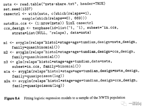
Figure 8.4 gives code for fitting a logistic regression model to the two-phase sample and to a case-control sample using both model-based and design-based analyses, and fitting a relative risk regression to the two-phase and nested case-control samples.
图8.4给出了代码同时使用基于模型和设计为基础的分析拟合逻辑回归模型的两相样品和病例 - 对照样品,和装配相对风险回归到两相和巢式病例对照样品。
The additional variables are s t a g e , the stage of the tumor, or how much it has spread (0-3); tumdiam, the size of the tumor, and age at diagnosis.
附加变量是 stage 、肿瘤的分期或扩散的程度 (0-3);tumdiam、肿瘤的大小和诊断时的年龄。
The estimates and standard errors are shown in Table 8.5.
估计值和标准误差如表 8.5 所示。
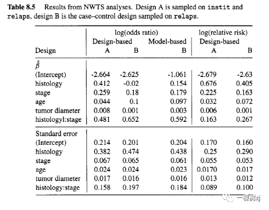
The first thing to note about the result is that the relative risks and odds ratios are quite different, especially for the histologyxstage interaction.
关于结果,首先要注意的是相对风险和优势比非常不同,尤其是对于组织学与分期的相互作用。
The reason is that relapse is quite common at advanced disease stages or with unfavorable histology.
原因是在疾病晚期或组织学不良时复发是很常见的。
The intercept estimate also differs substantially between the design-based and modelbased logistic regression analyses: the model-based estimate by ordinary logistic regression does not give the correct intercept.
基于设计和基于模型的逻辑回归分析的截距估计也有很大不同:普通逻辑回归的基于模型的估计不会给出正确的截距。
The bias should be equal to the log odds of being sampled for controls, which gives log(3246/669) = 1.58.
偏差应等于对照采样的对数几率,即 log(3246/669) = 1.58。
Correcting this bias gives an intercept of -2.84, in good agreement with the design-based analyses.
纠正这种偏差得到 -2.84 的截距,与基于设计的分析非常一致。
For both the log odds ratio and the log relative risk there is a noticeable gain in precision for interaction between histology and stage when sampling uses the surrogate exposure variable instit .
对于对数优势比和对数相对风险,当采样使用替代暴露变量 instit 时,组织学和分期之间相互作用的精确度显着提高。
There is relatively little impact on the standard errors of the other coefficients.
对其他系数的标准误影响相对较小。
The gain in precision is larger than the gain from using a model-based analysis of the case-control sample, and comes without having to make any additional assumptions.
精确度的增益大于使用基于模型的病例对照样本分析的增益,并且无需做出任何额外的假设。
As mentioned above, model-based approaches are also available for fitting linear and generalized linear models to two-phase samples.
正如上面提到的,基于模型的方法也可用于拟合线性和广义线性模型到两相的样品。
As with the case-control design, there is the potential for more precise estimates from the model-based approach and also the potential for bias when the model is misspecified.
作为与病例对照设计,对于从偏向基于模型的方法,也是潜在的更精确的估计潜在的当模型错误识别。
There has been a lot of theoretical research in this area, relatively little of which is published in ways accessible to the non-specialist.
在这方面有很多理论研究,其中以非专业人士可以访问的方式发表的相对较少。
The most general implementation of model-based analysis for two-phase studies is that of Scott and Wild [159], with R software and examples available from
用于两相研究中最一般实现基于模型的分析是,Scott和野生的[159],与[R软件和可得自实施例
8.4.3 Survival analysis
8.4.3 生存分析
The case-cohort design was developed by Prentice [127] as an alternative to a nested case-control design in a cohort study.
病例队列设计是由 Prentice [ 127]开发的,作为队列研究中嵌套病例对照设计的替代方案。
In the original case-cohort design the phasetwo sample consists of a subcohort chosen at the beginning of the study, augmented over time by all those who became cases.
在最初的病例队列设计中,第二阶段的样本由在研究开始时选择的子队列组成,随着时间的推移,所有成为病例的人都会增加。
The second phase is thus a stratified sample, stratified by case status.
因此,第二阶段是分层样本,按病例状态分层。
In contrast to the case-control design, where a given set of controls cannot readily be used for a different set of events, the same subcohort in a case-cohort can be used for studying cases of different diseases.
与病例对照设计相反,在病例对照设计中,一组给定的对照不容易用于不同的事件组,病例组中的同一亚组可用于研究不同疾病的病例。
Stratification on exposure variables is a natural extension, and was explored by Borgan et al[11] and by Samuelsenet al [146].
暴露变量的分层是一种自然延伸,Borgan等人[11] 和 Samuelsenet 人 [146]对此进行了探索。
Survival analysis based on case-cohort designs is currently more widely used than logistic regression based on two-phase samples.
基于案例的队列设计生存分析当前正在更广泛地比基于两相的样品logistic回归使用。
Recently published examples include examples of genotyping of stored DNA[90, 911, new biochemical assays of stored blood [55, 70, 1141, and new interviews and sample collection on the phase-two sample [87, 1651.
最近发表的例子包括对储存的 DNA 进行基因分型的例子 [90, 911,储存血液的新生化分析[55, 70, 1141,以及对第二阶段样本的新采访和样本收集 [87, 1651。
The case-cohort design is intended for studying time to an event such as relapse or death.
病例队列设计旨在研究复发或死亡等事件发生的时间。
In a regression model where the outcome variable is time to an event there is the complication that this event will usually not be observed for everyone in the cohort.
在结果变量是事件发生时间的回归模型中,复杂的是通常不会对队列中的每个人都观察到该事件。
If someone is alive at the end of follow-up their time to death is not known, but a lower bound is known, the current duration of follow-up.
如果有人在随访结束时还活着,他们的死亡时间是未知的,但下限是已知的,即当前的随访持续时间。
In this situation we say that the time to death is censured at the end of follow-up.
在这种情况下,我们说死亡时间在随访结束时受到谴责。
It is not possible to estimate the probability of the event or the mean time until the event from censored data.
不可能从删失数据估计事件发生的概率或事件发生前的平均时间。
Analyses of events and time-to-event in a cohort are most often based on the Co-x proportional hazards model.
队列中事件和事件发生时间的分析通常基于 Co-x 比例风险模型。
This is related to the logistic regression model, but models the rate of occurrence of events over time rather than the risk or probability of occurence.
这与逻辑回归模型有关,但对事件随时间的发生率进行建模,而不是对发生的风险或概率进行建模。
The rate (or “hazard”) for person i is written hi ( t ) , and by historical convention predictor variables are generically called z rather than x .
人i的比率(或“风险”)写为hi ( t ) ,并且按照历史惯例,预测变量通常称为z而不是x 。
The working model specifies the rate as a function of time
工作模型将速率指定为时间的函数
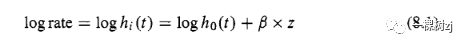
where log ho(t) is a set of intercepts for each time point, or equivalently
其中 log ho(t)是每个时间点的一组截距,或等效地
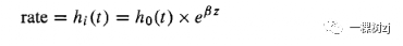
In this working model the effect of z on rate is multiplicative and does not change with time, leading to the name ‘proportional hazards model’.
在这个工作模型中,z对比率的影响是乘法的,不随时间变化,因此被称为“比例风险模型”。
The numbers efi are called hazard ratios, so the coefficients in the model, b, are the estimated log hazard ratios.
数字efi称为风险比,因此模型中的系数b是估计的对数风险比。
The collection of intercepts, ho(t) is called the baseline hazard.
截距的集合ho(t)称为基线风险。
The model in equation 8.1 does not explicitly mention the outcome variable.
方程 8.1 中的模型没有明确提及结果变量。
Operationally, the time to event outcome is represented by a combination of two variables in the data set: the duration of follow-up and the status at the end of followup.
在操作上,事件结果的时间由数据集中两个变量的组合表示:随访持续时间和随访结束时的状态。
In R these variables are packaged together with the Surv() function when they are supplied to a model formula.
在 R 中,这些变量在提供给模型公式时与Surv()函数一起打包。
Surv(time , status) represents observations with a follow-up duration of time and with status coded as 1 for those who had the event at the specified time and 0 for those who still had not had the event.
Surv(time , status)表示具有的随访时间观察时间与状态编码为1的那些谁在指定的有事件的时间和0对于那些谁仍然没有过的事件。
For detailed introductions to survival analysis see Breslow and Day [ 151 or Kleinbaum and Klein [76].
有关生存分析的详细介绍,请参阅 Breslow 和 Day [ 151] 或 Kleinbaum 和 Klein [76]。
The original methods for fitting the Cox model to case-cohort samples were designed so that the mathematical techniques available at the time could be used to study them.
拟合Cox模型来区分人群样本的原始方法旨在使该提供当时的数学技术可用于研究它们。
These mathematical techniques (Prentice[ 1271, Self and Prentice [ 160l)required the weight for each observation at each point in time to depend only on information collected before that point in time, even though data from the entire follow-up period was available.
这些数学技术(Prentice[1271,Self 和 Prentice [ 160l)要求每个时间点的每个观察的权重仅取决于该时间点之前收集的信息,即使整个随访期间的数据都是可用的。
Therneau & Li [168] describe how to implement these analyses in R and other statistical software.
Therneau & Li [168] 描述了如何在R和其他统计软件中实现这些分析。
Analyses based on a Cox model with two-phase sampling weights have now replaced the original methods.
基于具有两阶段采样权重的 Cox 模型的分析现已取代了原始方法。
Designbased methods for fitting the Cox model to complex samples were first described by Binder [9]and with more mathematical detail by Lin [95].
将 Cox 模型拟合到复杂样本的基于设计的方法首先由 Binder [9] 描述,并由 Lin [95] 描述了更多数学细节。
The asymptotic theory is substantially more complicated than for generalized linear models, and is still an active area of research, especially for two-phase designs [20,95].
渐近理论比广义线性模型复杂得多,并且仍然是一个活跃的研究领域,特别是对于两相设计 [20,95]。
8.4.4 Case-cohort designs in R
8.4.4病例队列设计的[R
The Wilms’ tumor population was used above in an example of logistic regression, but the time to relapse is also available, allowing case-cohort analyses to be simulated.
上面的逻辑回归示例中使用了 Wilms 的肿瘤群体,但也可以使用复发时间,从而可以模拟病例队列分析。
For the classical case-cohort analysis we take a sample from the cohort at the start of followup and then add all the cases to it.
对于经典的病例队列分析,我们在随访开始时从队列中抽取样本,然后将所有病例添加到其中。
If the expected event rate is about 1 in 7, giving about 650 expected cases, and we want about 650 non-cases, this means sampling a subcohort of 650 x 7/6 or about 750.
如果预期事件发生率约为 7 分之一,则给出大约 650 个预期案例,而我们想要大约 650 个非案例,这意味着对 650 x 7/6 或大约 750个子群组进行抽样。
For the one realization of the sampling scheme inFigure 8.5 there are 131 cases and 619 non-cases in the subcohort.
对于图 8.5 中抽样方案的一种实现,子队列中有 131 个案例和 619 个非案例。
Under this sampling design there are two sampled strata: those in the subcohort and those not in the subcohort.
在这种抽样设计下,有两个抽样层:在子队列中的层和不在子队列中的层。
The sampling probabilities are ~(211)= 750/3915 for the subcohort and ~ ( 2 1 1=) 1 for cases not in the subcohort.
对于子队列,抽样概率为~(211) = 750/3915,对于不在子队列中的案例,抽样概率为~ ( 2 1 1 = ) 1。
In Figure 8.5 the svycoxph() function fits the Cox proportional hazards model after the two-phase design has been set up.
在图8.5 中,svycoxph()函数在建立两阶段设计后拟合 Cox 比例风险模型。
The code also shows the classical modelbased analysis of Prentice [127] for these data.
该代码还显示了 Prentice [127] 对这些数据的经典基于模型的分析。
The cchO function (in the survival package) differs from svycoxph0 and twophase0 in that its input data are just the observations in the second-phase sample.
cchO功能(在survival包)从不同svycoxph()和twophase()在其输入数据仅仅是第二相样品中的观测。
The total cohort size is supplied as an additional argument.
总队列大小作为附加参数提供。
The two analyses do not give the same results even for point estimates.
即使对于点估计,这两种分析也不会给出相同的结果。
For example, the coefficient for histol is 0.96 with standard error 0.38 from cchO and 0.75 (std error 0.35) from svycoxph0.
例如,histol的系数为0.96,cchO 的标准误差为 0.38,svycoxph0 的标准误差为0.75(标准误差 0.35)。
The value using the entire sample is 0.59.
使用整个样本的值为0.59。
The differences between methods are unusually large in this example because the Cox model does not fit particularly well.
在此示例中,方法之间的差异异常大,因为 Cox 模型拟合得不是特别好。
Figure 8.6 shows an estimate of the coefficient of age as a function of time, produced with plot. cox. zph().
图 8.6 显示了作为时间函数的年龄系数的估计,用plot 生成。考克斯 zph() 。
The association is much stronger in the short term than later in time; the hazards are not proportional.
这种关联在短期内比后期强得多;危害不成比例。
The same is true for stage.
stage也是如此。
The different weighting for cases inside and outside the subcohort is aesthetically unattractive and will also result in a slight loss of efficiency.
子群组内部和外部案例的不同权重在美学上没有吸引力,也会导致效率略有下降。
We could instead have sampled all the cases and taken a sample of 619 non-cases, giving a two-phase design stratified on case status.
相反,我们可以对所有案例进行抽样,并从 619 个非案例中抽取样本,根据案例状态进行分层的两阶段设计。
Equivalently, we could post-stratify on case status.
同样,我们可以对案例状态进行后分层。
Either approach would result in weights of 3246/619 for non-cases and 1 for cases.
任何一种方法都会导致非案例的权重为 3246/619,案例的权重为 1。
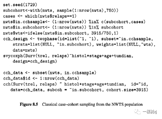
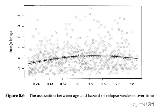
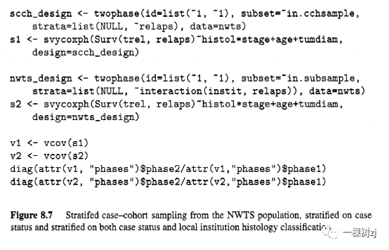
Figure 8.7 shows code with a sample stratified on case status.
图 8.7 显示了带有按案例状态分层的样本的代码。
The declaration of the design object is more straightforward here, as the weights can be computed by comparing the phase-one and phase-two samples.
此处设计对象的声明更为直接,因为可以通过比较第一阶段和第二阶段的样本来计算权重。
The stratified two-phase design analyzed with logistic regression in Figure 8.3 is also a stratified case-cohort design, and the same Cox model can be fitted, as shown.
图 8.3 中使用逻辑回归分析的分层两阶段设计也是分层病例队列设计,可以拟合相同的 Cox 模型,如图所示。
Figure 8.7 also shows how to examine the contributions of variance from each stage of sampling.
图 8.7 还显示了如何检查每个抽样阶段的方差贡献。
The variance matrix of a statistic computed from two-phase designs includes an attribute that gives the contributions of variance from each phase.
从两阶段设计计算的统计量的方差矩阵包括一个属性,该属性给出每个阶段的方差贡献。
In sampling from an existing cohort the first phase of sampling has been done in the past and cannot be changed.
在从现有队列中抽样时,抽样的第一阶段已在过去完成且无法更改。
The phase-one contribution to variance estimates the irreducible minimum uncertainty that would remain even if everyone in the cohort were included in the second phase of sampling.
第一阶段对方差的贡献估计了不可减少的最小不确定性,即使队列中的每个人都被包括在第二阶段的抽样中。
The phase-two contribution is the remainder of the variance, due to including only a subsample of the available cohort in the analysis.
第二阶段的贡献是方差的剩余部分,因为在分析中只包括可用队列的子样本。
Table 8.6 shows the estimated log hazard ratios and standard errors for the two models in Figure 8.7 and for a Cox model using the complete data.
表 8.6 显示了图 8.7 中两个模型和使用完整数据的 Cox 模型的估计对数风险比和标准误差。
The standard errors for the two case-cohort designs are divided into phase-one and phase-two contributions; the analysis of complete data has no phase-two component.
两个病例队列设计的标准误分为第一阶段和第二阶段贡献;完整数据的分析没有第二阶段的组成部分。
The estimated phase-one standard errors in all three model fits are estimating the same quantity and should be very similar, as indeed they are.
在所有三个模型拟合中估计的第一阶段标准误差估计的数量相同,应该非常相似,实际上它们是。
In the two stratified designs about 1/3 of the participants are included in phase two.
在两个分层设计中,大约 1/3 的参与者被包括在第二阶段。
If these 1/3 were a simple random sample the total variance would be about three times the phase-one variance, so the phase-two contribution would be about twice the phase-one contribution.
如果这 1/3 是一个简单的随机样本,则总方差大约是第一阶段方差的三倍,因此第二阶段的贡献将是第一阶段贡献的大约两倍。
In fact, across the coefficients in the model the estimated phase-two contributions range from 1.1 to 1.7 times the phase-one contributions for the design stratified only on case status and 70 to 90% of the phase-one contributions for the design stratified on both case status and local institution histologic classification.
事实上,在整个系数在模型所估计的相位两个贡献的范围从1.1至1.7倍的相,一个用于设计贡献分层仅在壳体的状态和的相位一个贡献70%至90%为分层的设计病例状态和当地机构组织学分类。
Both designs are better than random subsampling, and stratifying on histologic classification provides real improvement over stratifying only on case status.
两种设计都比随机子抽样更好,并且在组织学分类上分层比仅在病例状态上分层提供了真正的改进。
A more efficient model-based analysis is known in theory (Nan [115]), but it is difficult to program and no software is currently available.
一种更有效的基于模型的分析在理论上是已知的(Nan [115]),但它很难编程,目前还没有可用的软件。
8.5 using auxiliary information from phase one
8.5 使用第一阶段的辅助信息
In a two-phase subsampling design there are, in principle, three ways that auxiliary information could be used.
两相子采样设计中,原则上可以通过三种方式使用辅助信息。
Auxiliary variables whose totals are known for the whole population can be used to reweight either the phase-one sample or the phase-two subsample, and variables measured at phase one can be used to reweight the phasetwo subsample.
总人口已知的辅助变量可用于重新加权第一阶段样本或第二阶段子样本,并且在第一阶段测量的变量可用于重新加权第二阶段子样本。
There are typically few auxiliary variables available for the whole population, so we will focus on calibrating the second phase of sampling using auxiliary variables observed at phase one.
整个总体可用的辅助变量通常很少,因此我们将专注于使用在第一阶段观察到的辅助变量来校准采样的第二阶段。
One important difference between this setting and Chapter 7 is that the the phaseone data set includes individual-level information on auxiliary variables, not just totals, expanding the range of possible reweighting techniques.
此设置与第 7 章之间的一个重要区别是,phaseone 数据集包括有关辅助变量的个人级别信息,而不仅仅是总数,从而扩展了可能的重新加权技术的范围。
Another is that, since the auxiliary information will be available to the data analyst, the reweighting can easily be customized to a particular analysis.
另一个原因是,由于辅助信息可供数据分析师使用,因此可以轻松地针对特定分析定制重新加权。
A third difference is that, when sampling from an existing cohort, there may be a very large number of auxiliary variables available.
甲第三个区别是,从现有的队列采样时,有可能是可用的一个非常大的数量的辅助变量。
When estimating population means or totals, choosing auxiliary variables for two-phase designs follows much the same principles as in Chapter 7.
在估计总体均值或总数时,为两阶段设计选择辅助变量遵循与第 7 章中大致相同的原则。
For example, when estimating the prevalence of unfavorable histology in the case-cohort sample stratified only on r e l a p s , there would be an increase in precision if the phase-two sample were calibrated using inst it, which is correlated with histology.
例如,当估计仅在复发时分层的病例队列样本中不利组织学的发生率时,如果使用与组织学相关的inst it校准第二阶段样本,则精确度会提高。
As we saw in sections 7.3 and 7.4.1, it is more difficult to find auxiliary variables that increase the precision of subpopulation estimates or of regression parameter estimates.
正如我们在7.3和 7.4.1节中看到的,找到能够提高子总体估计或回归参数估计精度的辅助变量更加困难。
In particular, choosing variables that are correlated with the outcome variable or with predictor variables in a regression model is not very helpful.
特别是,选择与回归模型中的结果变量或预测变量相关的变量并不是很有帮助。
To see why this is the case and how to construct more effective auxiliary variables, we first go back to an artificial example with single-phase samples and population-level auxiliary variables, and then extend the lessons learnt to two-phase samples.
为了了解为什么会出现这种情况以及如何构建更有效的辅助变量,我们首先回到一个人工示例,其中包含单相样本和总体级辅助变量,然后将学到的经验扩展到两相样本。
8.5.1 Population calibration for regression models
8.5.1 回归模型的总体校准
Consider the regression model fitted to a sample from the Academic Performance Index population in section 7.4.1.
考虑适用于第7.4.1节中的学业成绩指数总体样本的回归模型。
The auxiliary variable in that example was the 1999 Academic Performance Index, which is highly correlated with the outcome variable, the 2000 Academic Performance Index.
该示例中的辅助变量是1999 年学业成绩指数,它与结果变量 2000 年学业成绩指数高度相关。
When estimating the mean 2000 API, population information on the 1999 API is helpful because a sample that, by chance, underestimates the mean 1999 API is likely to underestimate the mean 2000 API.
在估计 2000 API 均值时,1999 API 的总体信息很有帮助,因为偶然低估了1999 API均值的样本很可能会低估 2000 API 均值。
When estimating the slope of a regression line against student mobility the information is not directly useful: underestimating the mean API for high values of student mobility leads to an underestimate of the slope, but underestimating the mean API for low values of student mobility leads to an overestimate of the slope.
当根据学生流动性估计回归线的斜率时,该信息没有直接用处:低估学生流动性高值的平均 API 会导致对斜率的低估,但低估学生流动性低值的平均 API 会导致高估斜率。
Whether the slope is overestimated or underestimated is almost independent of whether the mean of the outcome variable is overestimated or underestimated.
斜率是高估还是低估几乎与结果变量的均值是高估还是低估无关。
For calibration to be useful in a regression model we need to construct a variable whose population mean or total approximates the estimated regression slope and then find auxiliary variables correlated with this constructed variable.
为了使校准在回归模型中有用,我们需要构建一个变量,其总体均值或总数接近估计的回归斜率,然后找到与该构建变量相关的辅助变量。
The theory of inj7uencefinction.s shows how to do this.
inj7uencefinction.s的理论展示了如何做到这一点。
The description in this section is fairly loose and heuristic, more details can be found in Breslow et al.[161].
本节中的描述相当松散和启发式,更多细节可以在 Breslow 等[1 61]中找到。
The influence function for an estimate b describes how the estimate changes when observations are added to or removed from the data.
估计值b的影响函数描述了在数据中添加或删除观察值时估计值如何变化。
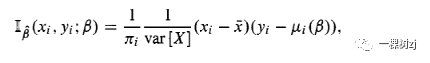
Write I[(Xi, yj ; ,6) for the influence function evaluated at data ( X i , y i ) and parameter value ,6.
为在数据(X i , yi )和参数值,6处评估的影响函数写出I[(Xi, yj ; ,6) 。
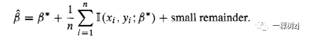
Also write ,6* for the true value of ,6, the value that would be obtained with complete population data.
还要写,6*作为,6的真值,即使用完整人口数据获得的值。
For nearly all estimates that are encountered in survey statistics, there is an explicitly computable influence function with the property
对于调查统计中遇到的几乎所有估计,都有一个明确的可计算的影响函数
Working out the influence function can be difficult for complex models, but the work has already been done for all the models and estimates we are using, since the linearization method of variance calculation requires these influence functions.
计算复杂模型的影响函数可能很困难,但我们使用的所有模型和估计都已经完成了工作,因为方差计算的线性化方法需要这些影响函数。
In linear, generalized linear, and proportional hazards regression models the influence functions evaluated at the observed data are just the At3 deletion diagnostics (exactly or approximately, there are some slight variations on how these are defined).
在线性、广义线性和比例风险回归模型中,对观察数据评估的影响函数只是At3删除诊断(确切地说或近似地,在如何定义这些方面存在一些细微的变化)。
Since any estimate can be approximated well by the population mean or total of its influence functions, good auxiliary variables for calibration will be highly correlated with these influence functions.
由于任何估计都可以通过总体均值或其影响函数的总和来很好地近似,因此用于校准的良好辅助变量将与这些影响函数高度相关。
The influence function Ib for a linear regression slope in a model with a single predictor variable is
具有单个预测变量的模型中线性回归斜率的影响函数Ib为
where Pi@) is the fitted value for individual i and X is the estimated population mean of X.
其中Pi@)是个体i的拟合值,X是X的估计总体均值。
If an auxiliary variable 2 is highly correlated with Y it will have a low correlation with Is, because the multiplier (xi - 2 ) can be negative or positive with about equal probability.
如果辅助变量2与Y高度相关,则它与Is 的相关性较低,因为乘数(xi - 2 )可以为负或正,概率大致相等。
If complete population data is available for Z and for X a better auxiliary variable can be constructed by fitting a linear regression of Z on X and taking the influence functions for this estimate.
如果Z和 X 的完整总体数据可用,则可以通过在 X 上拟合Z的线性回归并采用此估计的影响函数来构建更好的辅助变量。
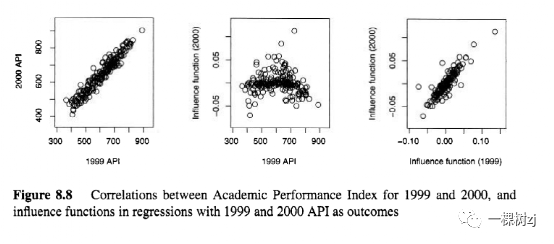
Figure 8.8 is based on the same example as in section 7.4.1.
图8.8基于与第 7.4.1 节中相同的示例。
It shows the relationship between 1999 and 2000 Academic Peformance Index, between 1999 API and the influence function for the coefficient of e l l , and between the influence functions for the coefficient of e l l using 1999 API and using 2000 API as the outcome variable.
它显示了 1999 年和 2000 年学术绩效指数之间、1999 年 API 和ell系数影响函数之间的关系,以及使用 1999 API 和使用 2000 API 作为结果变量的ell系数影响函数之间的关系。
The correlation between the two outcome variables is high, the correlation between the 2000 influence function and the 1999 outcome variable is low ( I = -0.05), and the correlation between the two influence functions is high ( r = 0.88).
两个结果变量之间的相关性较高,2000 年影响函数与 1999 年结果变量之间的相关性较低(I = -0.05),两个影响函数之间的相关性较高(r = 0.88)。
Figure 8.9 shows code and results for calibration using 1999 API directly and using it through the influence functions.
图 8.9 显示了直接使用 1999 API 并通过影响函数使用它的校准代码和结果。
The influence functions are constructed by fitting a population model with 1999 API as the outcome, then using df bet a (1 to extract the influence functions.
影响函数是通过拟合以 1999 API 作为结果的人口模型,然后使用df bet a (1提取影响函数。
The influence functions are then added as variables to the survey design object using update () , with match () used to work out which subset of the population collection of influence functions corresponds to the sample.
的影响的功能,然后作为变量调查设计对象使用添加更新() ,以匹配()用于影响函数对应的人口集合的哪个子集计算出到样品中。
The population totals for the influence functions are all zero, and c a l i b r a t e 0 reweights the sample to make the sample totals also zero.
影响函数的总体总数为零,校准 0重新加权样本以使样本总数也为零。
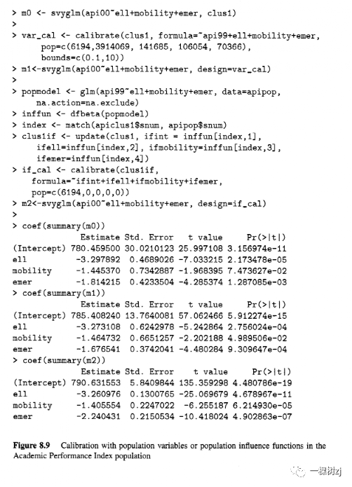
Calibration just using the variables api99, ell, mobility, and emer gives a substantial reduction in the intercept standard error, but has relatively little impact on the standard errors of the slope estimates.
仅使用变量api99、ell、mobility和emer 进行校准可大幅降低截距标准误差,但对斜率估计的标准误差影响相对较小。
Calibration using the influence functions further reduces the standard error of the intercept and reduces the standard errors of all the slope parameters by a factor of 2-3.
使用影响函数的校准进一步降低了截距的标准误差,并将所有斜率参数的标准误差降低了2-3倍。
8.5.2 Two-phase designs
8.5.2 两相设计
In the example above we assumed that all variables but one were known for the whole population, and at an individual level, not just as totals.
在上面的例子中,我们假设除了一个变量之外的所有变量对于整个总体来说都是已知的,并且在个体层面上,而不仅仅是总数。
This is unreasonable for sampling from a population, but is a typical situation when taking a two-phase sample from an existing cohort, where only a few new variables will be measured on the subsample.
这对于从总体中抽样来说是不合理的,但在从现有队列中抽取两阶段样本时,这是一种典型情况,在这种情况下,只会在子样本上测量几个新变量。
In the examples cited earlier of recent case-cohort analyses using stored DNA or stored blood, each model being fitted included only one or at most a few phase-two variables.
在前面引用的最近使用存储的DNA或存储的血液进行病例队列分析的示例中,每个拟合的模型仅包含一个或至多几个第二阶段变量。
Of more concern is whether the influence functions for the model of interest can be predicted effectively from phase-one information.
更令人担忧的是,是否可以从第一阶段信息有效地预测感兴趣模型的影响函数。
When the phase-two variables are common genetic polymorphisms being screened for association with a phase-one phenotype it is unlikely that any phase-one variables will provide useful information about the genotype and calibration is unlikely to be helpful.
当第二阶段变量是正在筛选与第一阶段表型关联的常见遗传多态性时,任何第一阶段变量都不太可能提供有关基因型的有用信息,校准也不太可能有帮助。
When an interaction between a phase-one and phase-two variable is of interest, calibration may be helpful.
当对第一阶段和第二阶段变量之间的相互作用感兴趣时,校准可能会有所帮助。
The most promising situation, however, is when there is a phase-one variable that is strongly correlated with the phase-two variable.
然而,最有希望的情况是当存在与第二阶段变量强相关的第一阶段变量时。
Strong correlations are most likely to exist when a phase-one variable is a crude measurement of some quantity and the phase-two variable is a more accurate measurement.
当第一阶段变量是对某个数量的粗略测量而第二阶段变量是更准确的测量时,最有可能存在强相关性。
Self-reported smoking at phase-one could be followed up by urinary cotinine screening at phase two.
在第一阶段自我报告的吸烟可以在第二阶段进行尿可替宁筛查。
“Has your doctor ever told you that you have high blood pressure?” could be followed up by blood pressure measurement and review of medications at phase two.
“你的医生有没有告诉你你有高血压?” 可以在第二阶段进行血压测量和药物审查。
A hospital discharge diagnosis of myocardial infarction, extracted from electronic records, could be followed up by review of detailed patient charts at phase two.
从电子记录中提取的心肌梗塞出院诊断可以通过在第二阶段查看详细的患者图表来跟进。
Another related possibility is that the phase-two variable is associated with some broad biological category of variables, such as the acute-phase inflammatory response, and that other biomarkers in the same category measured at phase one would be correlated with it.
另一种相关的可能性是,第二阶段变量与一些广泛的生物学变量相关,例如急性期炎症反应,并且在第一阶段测量的同一类别中的其他生物标志物将与其相关。
One reasonably general approach to constructing auxiliary variables based on influence functions is as follows [ 16]
基于影响函数构建辅助变量的一种合理通用的方法如下[ 16]
1. Build an imputation model to predict the phase-two variable from the phase-one variables
1.建立一个插补模型,从第一阶段的变量中预测第二阶段的变量
2. Fit a model to all of phase one, using the imputed value for observations that are not in the phase-two sample
2. 将模型拟合到所有第一阶段,使用不在第二阶段样本中的观测值的估算值
3. Use the influence functions from this model as auxiliary variables in calibration.
3.使用该模型的影响函数作为校准中的辅助变量。
In the API example in the previous subsection the first step was simplified: we imputed the 2000 API by the 1999 API.
在上一小节的 API 示例中,简化了第一步:我们通过 1999 API 估算了 2000 API。
Since the correlation between these variables was so high, a more sophisticated imputation model was unlikely to do any better.
由于这些变量之间的相关性如此之高,更复杂的插补模型不太可能做得更好。
Example: Wilms’ tumor
示例:维尔姆斯瘤
Breslow et al [17] used the Wilms’ tumor cohort data to illustrate this approach, in addition to reanalyzing data from a previously published case-cohort study in cardiovascular disease.
Breslow等人 [ 17] 使用 Wilms 的肿瘤队列数据来说明这种方法,此外还重新分析了先前发表的心血管疾病病例队列研究的数据。
The models fitted here are similar to those we used in that paper.
这里拟合的模型与我们在那篇论文中使用的模型相似。
The first step is to construct an imputation model for the central lab histologic classification.
第一步是为中心实验室组织学分类构建一个插补模型。
This model is fitted to the phase-two sample, but uses only predictor variables from phase one.
该模型适用于第二阶段样本,但仅使用第一阶段的预测变量。
The most important predictor will be the local lab classification, but there may be additional information in other variables.
最重要的预测因素将是当地实验室分类,但其他变量中可能还有其他信息。
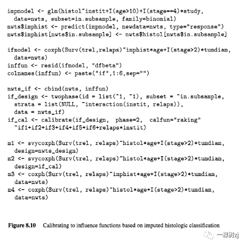
The imputation model in Figure 8.10 follows Kulich and Lin [85] .
图 8.10 中的插补模型遵循 Kulich 和 Lin [85]。
The predicted values are extracted from the logistic regression model with predict 0, into a variable imphist and the known central-lab histologic classification is used for the phase-two subsample where it is known.
预测值从预测值为 0的逻辑回归模型中提取到变量imhist 中,并且已知的中心实验室组织学分类用于已知的第二阶段子样本。
The next step is to fit a model to the whole phase-one sample using the imputed histology variable, to provide influence functions that will be used as auxiliary variables.
下一步是使用估算的组织学变量将模型拟合到整个第一阶段样本,以提供将用作辅助变量的影响函数。
The influence functions for a Cox model are extracted using the resid() function.
使用resid()函数提取 Cox 模型的影响函数。
These influence functions are added to the nwts data set and a new survey object is defined.
这些影响函数被添加到nwts数据集中,并定义了一个新的调查对象。
Finally, this new survey object is calibrated using the influence functions as auxiliary variables.
最后,使用影响函数作为辅助变量校准这个新的调查对象。
The call to calibrate() specifies phase=2, indicating that the phase-two subsample is being calibrated to the phase-one sample.
对calibrate()的调用指定phase=2,表明第二阶段子样本正在被校准为第一阶段样本。
It is not necessary to specify totals for the auxiliary variables as the full phase-one data are stored in the survey design object and these totals can readily be computed.
没有必要指定辅助变量的总数,因为完整的第一阶段数据存储在调查设计对象中,并且这些总数可以很容易地计算出来。
Raking calibration is used to ensure non-negative weights, which the Cox regression functions require.
Raking 校准用于确保非负权重,这是 Cox 回归函数所需的。
The first two models, mi and m2, are fitted to the two-phase sample using sampling weights and calibrated weights, respectively.
前两个模型mi和m2分别使用采样权重和校准权重拟合到两相样本。
Since this procedure requires imputing the central-lab histologic classification for all children in the study, another approach would be to use this imputed value directly as a predictor and fit an unweighted model to the whole sample (m3).
由于此过程需要对研究中所有儿童的中心实验室组织学分类进行插补,因此另一种方法是直接使用该插补值作为预测变量,并将未加权模型拟合到整个样本(m3)。
This would be a standard choice if the analysis were viewed as a measurement-error problem.
如果分析被视为测量误差问题,这将是一个标准选择。
The coefficient estimates are slightly biased even if the imputation model is fits well, though not enough to cause practical problems in interpretation.
即使插补模型拟合良好,系数估计也略有偏差,但不足以在解释中引起实际问题。
The bias can be more serious when the imputation model fits poorly.
当插补模型拟合不佳时,偏差可能会更严重。
Table 8.7 shows the coefficient estimates and standard errors from these three models and model m 4 that uses the complete data on central lab histology.
表8.7显示了这三个模型和使用中央实验室组织学完整数据的模型m 4的系数估计值和标准误差。
Both raking and imputation reduce the standard errors.
倾斜和插补都减少了标准误差。
This is especially true for variables that are observed for everyone in the sample, where the standard errors are close to those that would be obtained with complete data.
对于样本中每个人都观察到的变量来说尤其如此,其中标准误与使用完整数据获得的标准误很接近。
The results are very similar for raking and direct imputation, which tends to be the case when the imputation model is good.
耙式和直接插补的结果非常相似,当插补模型良好时往往是这种情况。
The raking approach has the additional advantage of always being valid, without any assumptions about models, and of always being at least as accurate as the two-phase analysis based on sampling weights.
扒出方法始终是有效的,没有关于模型的任何假设的额外的优势,至少总是被精确基于两阶段分析的抽样权重。
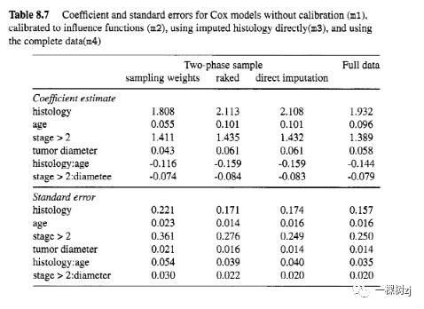
On the other hand, in small phase-two samples or with low event rates direct imputation has the advantage of not requiring any events to occur in the phase-two subsample.
另一方面,在较小的第二阶段样本或具有低事件率的情况下,直接插补的优点是不需要在第二阶段子样本中发生任何事件。
For example, the Women’s Health Initiative trial measured protein and energy intake in using biomarkers in a small subsample of participants chosen at the start of the study [ 1 181.
例如,妇女健康倡议试验在研究开始时选择的一小部分参与者中使用生物标志物测量了蛋白质和能量摄入量[ 1181。
Only a handful of heart disease or cancer events would be expected in this subsample and a two-phase sampling approach would be ineffective.
在这个子样本中,预计只有少数心脏病或癌症事件,两阶段抽样方法是无效的。
8.5.3 Some history of the two-phase calibration estimator
8.5.3一些历史的两相位校准估计
Shdal and Swensson [150] reviewed two-phase estimation, including regression estimators for the population total using either population or phase-one auxiliary variables, but they did not consider estimating other statistics.
Shdal 和 Swensson [ 150] 回顾了两阶段估计,包括使用总体或第一阶段辅助变量的总体回归估计量,但他们没有考虑估计其他统计量。
Robins, Rotnitzky, and Zhao [137] characterized all the valid estimators for regression coefficients in a two-phase design and showed how (in theory) the most efficient design-based and model-based estimators were constructed.
Robins、Rotnitzky 和 Zhao [ 137] 描述了两阶段设计中回归系数的所有有效估计量,并展示了如何(理论上)构建最有效的基于设计和基于模型的估计量。
Their “Augmented Inverse-Probability Weighted” (AIPW) estimators are related to design-based calibration estimators, and the most efficient AIPW estimators corresponds to the calibration estimator with the optimal set of auxiliary variables.
他们的“增强逆概率加权”(AIPW)估计都与基于设计的校准估计,最有效的AIPW估计对应于具有最佳的组中的校准估计的辅助变量。
In practice it is not feasible to construct this estimator, since it involves expected values taken over an unknown population distribution.
实际上,构建这个估计量是不可行的,因为它涉及对未知人口分布的期望值。
Breslow and Chatterjee [13] and Borgan et al [11] described post-stratification for regression models in two-phase samples, for logistic regression and Cox regression respectively.
Breslow 和 Chatterjee [ 13] 以及 Borgan 等人 [11] 描述了两相样本中回归模型的后分层,分别用于逻辑回归和 Cox 回归。
Kulich and Lin[85] constructed a complicated ratio-type estimator based on adjusting the sampling weights separately for each time point and each predictor variable.
Kulich 和Lin[85]基于对每个时间点和每个预测变量分别调整采样权重构建了一个复杂的比率型估计器。
The strategy of imputing the phase-two variable and using influence functions as auxiliary variables is a simpler version of their approach.
输入第二阶段变量并使用影响函数作为辅助变量的策略是他们方法的更简单版本。
Breslow and Lumley and coworkers [16, 17] describe applications and theory for the approach based on influence functions.
Breslow 和 Lumley 及其同事 [16, 17] 描述了基于影响函数的方法的应用和理论。
Mark and Katki [103] followed the approach of Robins and colleagues more directly and worked out the design-based estimator that would be optimal under particular parametric models.
Mark 和 Katki [ 103] 更直接地遵循 Robins 及其同事的方法,并计算出在特定参数模型下最佳的基于设计的估计量。
This is implemented it in the R package NestedCohort [71].
这是在 R 包NestedCohort [71] 中实现的。
NestedCohort has the advantage of being able to compute standard errors for survival curves, which survey did not implement at the time of writing.
NestedCohort的优势在于能够计算生存曲线的标准误差,而在撰写本文时该调查并未实施。
All these approaches give similar results for examples based on the Wilms’ tumor population; it is not clear how they compare in general.
对于基于 Wilms 肿瘤群体的示例,所有这些方法都给出了类似的结果;目前尚不清楚它们的总体比较情况。
Until very recently there has been no overlap between the survey literature based on calibration or GREG estimation and the biostatistics literature descended from Robins, Rotnitzky, and Zhao; as of mid-2008 the Web of Science citation system listed no paper that cited both [137] and one of [40,41, 150].
直到最近,基于校准或 GREG 估计的调查文献与来自 Robins、Rotnitzky 和 Zhao 的生物统计学文献之间还没有重叠;截至 2008 年年中,Web of Science 引文系统未列出同时引用 [137] 和 [40,41, 150] 之一的论文
