本文包括:
SCIentific PYthon 简介插值插值示例线性插值多项式插值径向基函数径向基函数插值高维 `RBF` 插值
SCIentific PYthon 简介
Ipython
提供了一个很好的解释器界面。
Matplotlib
提供了一个类似 Matlab
的画图工具。
Numpy
提供了 ndarray
对象,可以进行快速的向量化计算。
Scipy
是 Python
中进行科学计算的一个第三方库,以 Numpy
为基础。
Pandas
是处理时间序列数据的第三方库,提供一个类似 R
语言的环境。
StatsModels
是一个统计库,着重于统计模型。
Scikits
以 Scipy
为基础,提供如 scikits-learn
机器学习和scikits-image
图像处理等高级用法。
Scipy
由不同科学计算领域的子模块组成:
| 子模块 | 描述 |
|---|---|
cluster | 聚类算法 |
constants | 物理数学常数 |
fftpack | 快速傅里叶变换 |
integrate | 积分和常微分方程求解 |
interpolate | 插值 |
io | 输入输出 |
linalg | 线性代数 |
odr | 正交距离回归 |
optimize | 优化和求根 |
signal | 信号处理 |
sparse | 稀疏矩阵 |
spatial | 空间数据结构和算法 |
special | 特殊方程 |
stats | 统计分布和函数 |
weave | C/C++ 积分 |
在使用 Scipy
之前,为了方便,假定这些基础的模块已经被导入:
1import numpy as np
2import scipy as sp
3import matplotlib as mpl
4import matplotlib.pyplot as plt
使用 Scipy 中的子模块时,需要分别导入:
1from scipy import linalg, optimize
对于一些常用的函数,这些在子模块中的函数可以在 scipy
命名空间中调用。另一方面,由于 Scipy
以 Numpy
为基础,因此很多基础的 Numpy
函数可以在scipy
命名空间中直接调用。
我们可以使用 numpy
中的 info
函数来查看函数的文档:
1np.info(optimize.fmin)
  1 fmin(func, x0, args=(), xtol=0.0001, ftol=0.0001, maxiter=None, maxfun=None,
  2      full_output=0, disp=1, retall=0, callback=None, initial_simplex=None)
  3
  4Minimize a function using the downhill simplex algorithm.
  5
  6This algorithm only uses function values, not derivatives or second
  7derivatives.
  8
  9Parameters
 10----------
 11func : callable func(x,*args)
 12    The objective function to be minimized.
 13x0 : ndarray
 14    Initial guess.
 15args : tuple, optional
 16    Extra arguments passed to func, i.e. ``f(x,*args)``.
 17xtol : float, optional
 18    Absolute error in xopt between iterations that is acceptable for
 19    convergence.
 20ftol : number, optional
 21    Absolute error in func(xopt) between iterations that is acceptable for
 22    convergence.
 23maxiter : int, optional
 24    Maximum number of iterations to perform.
 25maxfun : number, optional
 26    Maximum number of function evaluations to make.
 27full_output : bool, optional
 28    Set to True if fopt and warnflag outputs are desired.
 29disp : bool, optional
 30    Set to True to print convergence messages.
 31retall : bool, optional
 32    Set to True to return list of solutions at each iteration.
 33callback : callable, optional
 34    Called after each iteration, as callback(xk), where xk is the
 35    current parameter vector.
 36initial_simplex : array_like of shape (N + 1, N), optional
 37    Initial simplex. If given, overrides `x0`.
 38    ``initial_simplex[j,:]`` should contain the coordinates of
 39    the j-th vertex of the ``N+1`` vertices in the simplex, where
 40    ``N`` is the dimension.
 41
 42Returns
 43-------
 44xopt : ndarray
 45    Parameter that minimizes function.
 46fopt : float
 47    Value of function at minimum: ``fopt = func(xopt)``.
 48iter : int
 49    Number of iterations performed.
 50funcalls : int
 51    Number of function calls made.
 52warnflag : int
 53    1 : Maximum number of function evaluations made.
 54    2 : Maximum number of iterations reached.
 55allvecs : list
 56    Solution at each iteration.
 57
 58See also
 59--------
 60minimize: Interface to minimization algorithms for multivariate
 61    functions. See the 'Nelder-Mead' `method` in particular.
 62
 63Notes
 64-----
 65Uses a Nelder-Mead simplex algorithm to find the minimum of function of
 66one or more variables.
 67
 68This algorithm has a long history of successful use in applications.
 69But it will usually be slower than an algorithm that uses first or
 70second derivative information. In practice it can have poor
 71performance in high-dimensional problems and is not robust to
 72minimizing complicated functions. Additionally, there currently is no
 73complete theory describing when the algorithm will successfully
 74converge to the minimum, or how fast it will if it does. Both the ftol and
 75xtol criteria must be met for convergence.
 76
 77Examples
 78--------
 79>>> def f(x):
 80...     return x**2
 81
 82>>> from scipy import optimize
 83
 84>>> minimum = optimize.fmin(f, 1)
 85Optimization terminated successfully.
 86         Current function value: 0.000000
 87         Iterations: 17
 88         Function evaluations: 34
 89>>> minimum[0]
 90-8.8817841970012523e-16
 91
 92References
 93----------
 94.. [1] Nelder, J.A. and Mead, R. (1965), "A simplex method for function
 95       minimization", The Computer Journal, 7, pp. 308-313
 96
 97.. [2] Wright, M.H. (1996), "Direct Search Methods: Once Scorned, Now
 98       Respectable", in Numerical Analysis 1995, Proceedings of the
 99       1995 Dundee Biennial Conference in Numerical Analysis, D.F.
100       Griffiths and G.A. Watson (Eds.), Addison Wesley Longman,
101       Harlow, UK, pp. 191-208.
可以用 lookfor
来查询特定关键词相关的函数:
1np.lookfor("resize array")
 1Search results for 'resize array'
 2---------------------------------
 3numpy.chararray.resize
 4    Change shape and size of array in-place.
 5numpy.ma.resize
 6    Return a new masked array with the specified size and shape.
 7numpy.resize
 8    Return a new array with the specified shape.
 9numpy.chararray
10    chararray(shape, itemsize=1, unicode=False, buffer=None, offset=0,
11numpy.memmap
12    Create a memory-map to an array stored in a *binary* file on disk.
13numpy.squeeze
14    Remove single-dimensional entries from the shape of an array.
15numpy.expand_dims
16    Expand the shape of an array.
17numpy.ma.MaskedArray.resize
18    .. warning::
还可以指定查找的模块:
1np.lookfor("remove path", module="os")
1Search results for 'remove path'
2--------------------------------
3os.removedirs
4    removedirs(name)
5os.walk
6    Directory tree generator.
插值
1import numpy as np
2import matplotlib.pyplot as plt
3%matplotlib inline
设置 Numpy
浮点数显示格式:
1np.set_printoptions(precision=2, suppress=True)
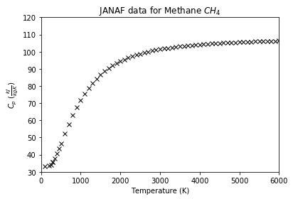
从文本中读入数据,数据来自 http://kinetics.nist.gov/janaf/html/C-067.txt ,保存为结构体数组:
1data = np.genfromtxt("JANAF_CH4.txt",
2                  delimiter="\t", # TAB 分隔
3                  skip_header=1,     # 忽略首行
4                  names=True,     # 读入属性
5                  missing_values="INFINITE",  # 缺失值
6                  filling_values=np.inf)      # 填充缺失值
显示部分数据:
1for row in data[:7]:
2    print(f"{row['TK']}\t{row['Cp']}")
3print("...\t...")
10.0    0.0
2100.0    33.258
3200.0    33.473
4250.0    34.216
5298.15    35.639
6300.0    35.708
7350.0    37.874
8...    ...
绘图:
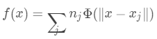
1p = plt.plot(data['TK'], data['Cp'], 'kx')
2t = plt.title("JANAF data for Methane $CH_4$")
3a = plt.axis([0, 6000, 30, 120])
4x = plt.xlabel("Temperature (K)")
5y = plt.ylabel(r"$C_p$ ($\frac{kJ}{kg K}$)")
插值示例
假设我们要对这组数据进行插值。
先导入一维插值函数 interp1d
:
1interp1d(x, y)
1from scipy.interpolate import interp1d
1ch4_cp = interp1d(data['TK'], data['Cp'])
interp1d
的返回值可以像函数一样接受输入,并返回插值的结果。
单个输入值,注意返回的是数组:
1ch4_cp(382.2)
1array(39.57)
输入数组,返回的是对应的数组:
1ch4_cp([32.2,323.2])
1array([10.71, 36.71])
默认情况下,输入值要在插值允许的范围内,否则插值会报错:
1ch4_cp(8752)
 1---------------------------------------------------------------------------
 2
 3ValueError                                Traceback (most recent call last)
 4
 5<ipython-input-10-737d7cfff1c9> in <module>()
 6----> 1 ch4_cp(8752)
 7
 8
 9D:\Anaconda3\lib\site-packages\scipy\interpolate\polyint.py in __call__(self, x)
10     77         """
11     78         x, x_shape = self._prepare_x(x)
12---> 79         y = self._evaluate(x)
13     80         return self._finish_y(y, x_shape)
14     81
15
16
17D:\Anaconda3\lib\site-packages\scipy\interpolate\interpolate.py in _evaluate(self, x_new)
18    662         y_new = self._call(self, x_new)
19    663         if not self._extrapolate:
20--> 664             below_bounds, above_bounds = self._check_bounds(x_new)
21    665             if len(y_new) > 0:
22    666                 # Note fill_value must be broadcast up to the proper size
23
24
25D:\Anaconda3\lib\site-packages\scipy\interpolate\interpolate.py in _check_bounds(self, x_new)
26    694                              "range.")
27    695         if self.bounds_error and above_bounds.any():
28--> 696             raise ValueError("A value in x_new is above the interpolation "
29    697                              "range.")
30    698
31
32
33ValueError: A value in x_new is above the interpolation range.
34
但我们可以通过参数设置允许超出范围的值存在,不过由于超出范围,所以插值的输出是非法值:
1ch4_cp = interp1d(data['TK'], data['Cp'], bounds_error=False)
2ch4_cp(8752)
1array(nan)
可以使用指定值替代这些非法值:
1ch4_cp = interp1d(data['TK'],
2                  data['Cp'],
3                  bounds_error=False,
4                  fill_value=-999.25)
5ch4_cp(8752)
1array(-999.25)
线性插值
interp1d
默认的插值方法是线性,关于线性插值的定义,请参见:
维基百科-线性插值:https://zh.wikipedia.org/wiki/%E7%BA%BF%E6%80%A7%E6%8F%92%E5%80%BC
百度百科-线性插值:http://baike.baidu.com/view/4685624.htm
其基本思想是,已知相邻两点 对应的值 ,那么对于  之间的某一点 ,线性插值对应的值 满足:点 在
  所形成的线段上。
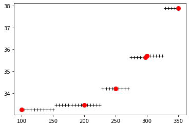
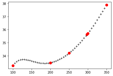
应用线性插值:
1T = np.arange(100,355,5)
2plt.plot(T, ch4_cp(T), "+k")
3p = plt.plot(data['TK'][1:7], data['Cp'][1:7], 'ro', markersize=8)
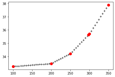
其中红色的圆点为原来的数据点,黑色的十字点为对应的插值点,可以明显看到,相邻的数据点的插值在一条直线上。
多项式插值
我们可以通过 kind
参数来调节使用的插值方法,来得到不同的结果:
nearest
最近邻插值zero
0阶插值linear
线性插值quadratic
二次插值cubic
三次插值4,5,6,7
更高阶插值
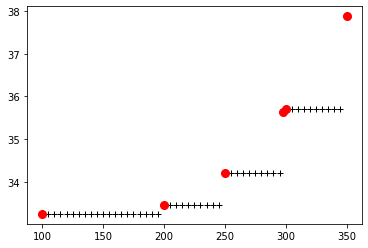
最近邻插值:
1cp_ch4 = interp1d(data['TK'], data['Cp'], kind="nearest")
2p = plt.plot(T, cp_ch4(T), "k+")
3p = plt.plot(data['TK'][1:7], data['Cp'][1:7], 'ro', markersize=8)
0阶插值:
1cp_ch4 = interp1d(data['TK'], data['Cp'], kind="zero")
2p = plt.plot(T, cp_ch4(T), "k+")
3p = plt.plot(data['TK'][1:7], data['Cp'][1:7], 'ro', markersize=8)
二次插值:
1cp_ch4 = interp1d(data['TK'], data['Cp'], kind="quadratic")
2p = plt.plot(T, cp_ch4(T), "k+")
3p = plt.plot(data['TK'][1:7], data['Cp'][1:7], 'ro', markersize=8)
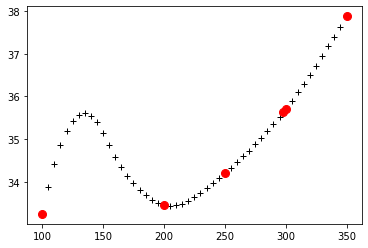
三次插值:
1cp_ch4 = interp1d(data['TK'], data['Cp'], kind="cubic")
2p = plt.plot(T, cp_ch4(T), "k+")
3p = plt.plot(data['TK'][1:7], data['Cp'][1:7], 'ro', markersize=8)
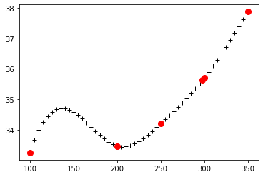
事实上,我们可以使用更高阶的多项式插值,只要将 kind
设为对应的数字(大于3时必须为奇数):
五次多项式插值:
1cp_ch4 = interp1d(data['TK'], data['Cp'], kind=5)
2p = plt.plot(T, cp_ch4(T), "k+")
3p = plt.plot(data['TK'][1:7], data['Cp'][1:7], 'ro', markersize=8)
可以参见:
维基百科-多项式插值:https://zh.wikipedia.org/wiki/%E5%A4%9A%E9%A1%B9%E5%BC%8F%E6%8F%92%E5%80%BC
百度百科-插值法:http://baike.baidu.com/view/754506.htm
对于二维乃至更高维度的多项式插值:
1from scipy.interpolate import interp2d, interpnd
其使用方法与一维类似。
径向基函数
关于径向基函数,可以参阅:
维基百科-Radial basis fucntion:https://en.wikipedia.org/wiki/Radial_basis_function
径向基函数,简单来说就是点 处的函数值只依赖于 与某点 的距离:
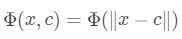
1x = np.linspace(-3,3,100)
常用的径向基(RBF
)函数有:
高斯函数:
1plt.plot(x, np.exp(-1 * x **2))
2t = plt.title("Gaussian")
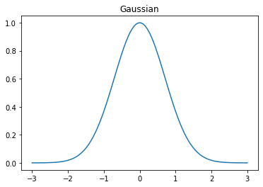
Multiquadric函数:
1plt.plot(x, np.sqrt(1 + x **2))
2t = plt.title("Multiquadric")
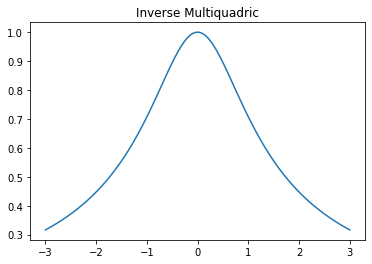
Inverse Multiquadric
函数:
1plt.plot(x, 1. / np.sqrt(1 + x **2))
2t = plt.title("Inverse Multiquadric")
径向基函数插值
对于径向基函数,其插值的公式为:
我们通过数据点 来计算出 的值,来计算 处的插值结果。
1from scipy.interpolate.rbf import Rbf
使用 multiquadric
核的:
1cp_rbf = Rbf(data['TK'], data['Cp'], function = "multiquadric")
2plt.plot(data['TK'], data['Cp'], 'k+')
3p = plt.plot(data['TK'], cp_rbf(data['TK']), 'r-')
使用 gaussian
核:
1cp_rbf = Rbf(data['TK'], data['Cp'], function = "gaussian")
2plt.plot(data['TK'], data['Cp'], 'k+')
3p = plt.plot(data['TK'], cp_rbf(data['TK']), 'r-')
使用 nverse_multiquadric
核:
1cp_rbf = Rbf(data['TK'], data['Cp'], function = "inverse_multiquadric")
2plt.plot(data['TK'], data['Cp'], 'k+')
3p = plt.plot(data['TK'], cp_rbf(data['TK']), 'r-')
不同的 RBF
核的结果也不同。
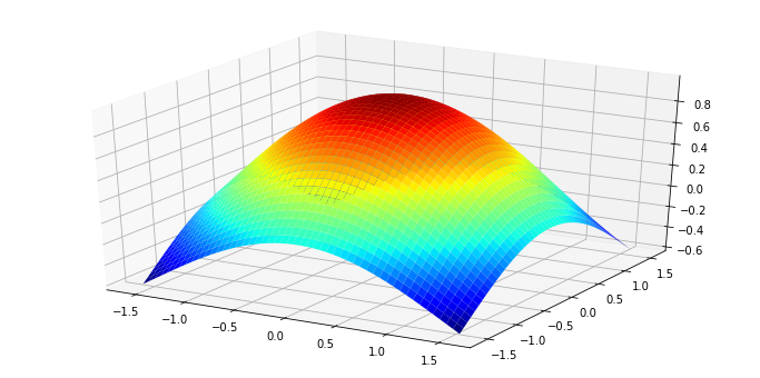
高维 `RBF` 插值
1from mpl_toolkits.mplot3d import Axes3D
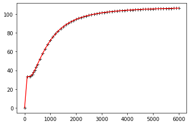
三维数据点:
1x, y = np.mgrid[-np.pi/2:np.pi/2:5j, -np.pi/2:np.pi/2:5j]
2z = np.cos(np.sqrt(x**2 + y**2))
1fig = plt.figure(figsize=(12,6))
2ax = fig.gca(projection="3d")
3ax.scatter(x,y,z)
1<mpl_toolkits.mplot3d.art3d.Path3DCollection at 0x1a03c1d0>
3维 RBF
插值:
1zz = Rbf(x, y, z)
1xx, yy = np.mgrid[-np.pi/2:np.pi/2:50j, -np.pi/2:np.pi/2:50j]
2fig = plt.figure(figsize=(12,6))
3ax = fig.gca(projection="3d")
4ax.plot_surface(xx,yy,zz(xx,yy),rstride=1, cstride=1, cmap=plt.cm.jet)
1<mpl_toolkits.mplot3d.art3d.Poly3DCollection at 0x1a20a828>