最小化函数minimize 函数Rosenbrock 函数优化方法BFGS 算法Nelder-Mead Simplex 算法Powell 算法

最小化函数

minimize 函数

%pylab inline
set_printoptions(precision=3, suppress=True)

plt.rcParams["font.family"] = "SimHei"
plt.rcParams["axes.unicode_minus"] = False

Populating the interactive namespace from numpy and matplotlib

已知斜抛运动的水平飞行距离公式：

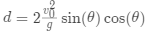
• 水平飞行距离

• 初速度大小

• 重力加速度

• 抛出角度

希望找到使 最大的角度 。

定义距离函数：

def dist(theta, v0):
    """计算以V0(m/s)初速度在θ度发射的弹丸的飞行距离"""
    g = 9.8
    theta_rad = pi * theta / 180
    return 2 * v0**2 / g * sin(theta_rad) * cos(theta_rad)

print("optimal dist:", dist(45, 1.))

optimal dist: 0.1020408163265306

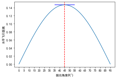
theta = linspace(0, 90, 90)
v0 = 1.2
optimal_dist = dist(45, v0)
print("optimal dist:", optimal_dist)
p = plot(theta, dist(theta, v0))
plt.xlabel(r'抛出角度$\theta (^{\circ})$')
plt.xticks(np.arange(0, 95, 5))
plt.ylabel('水平飞行距离')
plt.hlines(optimal_dist, xmin=35, xmax=55, colors="b")
plt.axvline(45, ymin=0, ymax=1, color="r", ls="--")
plt.show()

optimal dist: 0.14693877551020407

因为 Scipy
 提供的是最小化方法，所以最大化距离就相当于最小化距离的负数：

def neg_dist(theta, v0):
    return -1 * dist(theta, v0)

导入 scipy.optimize.minimize
：

from scipy.optimize import minimize
result = minimize(neg_dist, x0=50, args=(1, ))
print(f"optimal angle = {result.x[0]:.1f} degrees")

optimal angle = 45.0 degrees

minimize
 接受三个参数：第一个是要优化的函数，第二个是初始猜测值，第三个则是优化函数的附加参数，默认 minimize
 将优化函数的第一个参数作为优化变量，所以第三个参数输入的附加参数从优化函数的第二个参数开始。

查看返回结果：

print(result)

      fun: -0.10204080675612252
 hess_inv: array([[8095.275]])
      jac: array([-0.])
  message: 'Optimization terminated successfully.'
     nfev: 27
      nit: 3
     njev: 9
   status: 0
  success: True
        x: array([44.988])

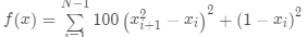
Rosenbrock 函数

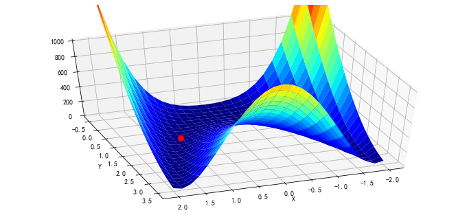
Rosenbrock 函数是一个用来测试优化函数效果的一个非凸函数：

导入该函数：

from scipy.optimize import rosen
from mpl_toolkits.mplot3d import Axes3D

使用 N = 2
 的 Rosenbrock 函数：

x, y = meshgrid(np.linspace(-2,2,25), np.linspace(-0.5,3.5,25),sparse=True)
# x, y
z = rosen([x,y])
# 图像和最低点 (1,1)：
rosen([1,1])

0.0

图像和最低点 (1,1)
：

fig = figure(figsize=(12, 5.5))
ax = fig.gca(projection="3d")
ax.azim = 70
ax.elev = 48
ax.set_xlabel("X")
ax.set_ylabel("Y")
ax.set_zlim((0, 1000))
p = ax.plot_surface(x, y, z, rstride=1, cstride=1, cmap=cm.jet)
# 图像和最低点 (1,1)：
rosen_min = ax.plot([1], [1], [0], "ro", zorder=9999, markersize=8)

传入初始值：

x0 = [1.3, 1.6, -0.5, -1.8, 0.8]
result = minimize(rosen, x0)
print(result.x)

[-0.962  0.936  0.881  0.778  0.605]

随机给定初始值：

x0 = np.random.randn(10)
result = minimize(rosen, x0)
print(x0)
print(result.x)

[ 0.374  1.879 -0.407 -0.989 -1.432  1.893  0.339 -0.322 -1.716 -1.614]
[1. 1. 1. 1. 1. 1. 1. 1. 1. 1.]

对于 N > 3
，函数的最小值为 ，不过有一个局部极小值点 ，所以随机初始值如果选的不好的话，有可能返回的结果是局部极小值点：

优化方法

BFGS 算法

minimize
 函数默认根据问题是否有界或者有约束，使用 'BFGS', 'L-BFGS-B', 'SLSQP'
 中的一种。

可以查看帮助来得到更多的信息：

minimize?

默认没有约束时，使用的是 BFGS 方法。

利用 callback
 参数查看迭代的历史：

x0 = [-1.5, 4.5]
xi = [x0]
result = minimize(rosen, x0, callback=xi.append)
xi = np.asarray(xi)
print(xi.shape)
print(result.x)
print("in {} function evaluations.".format(result.nfev))

(48, 2)
[1. 1.]
in 252 function evaluations.

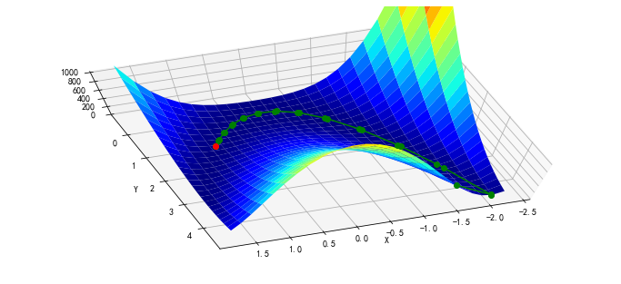
绘图显示轨迹：

x, y = meshgrid(np.linspace(-2.3, 1.75, 25),
                np.linspace(-0.5, 4.5, 25),
                sparse=True)
z = rosen([x, y])
fig = figure(figsize=(12, 5.5))
ax = fig.gca(projection="3d")
ax.azim = 70
ax.elev = 75
ax.set_xlabel("X")
ax.set_ylabel("Y")
ax.set_zlim((0, 1000))
p = ax.plot_surface(x, y, z, rstride=1, cstride=1, cmap=cm.jet)
intermed = ax.plot(xi[:, 0], xi[:, 1], rosen(xi.T), "g-o", zorder=99)
rosen_min = ax.plot([1], [1], [0], "ro", zorder=100)

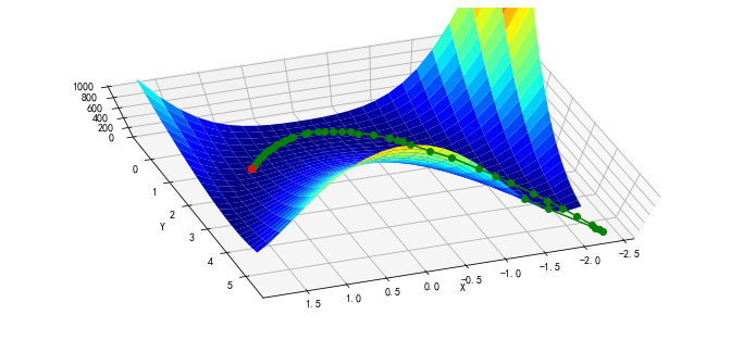
BFGS
 需要计算函数的 Jacobian 矩阵：

给定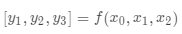 

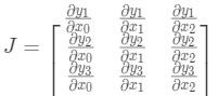
在我们的例子中

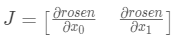
导入 rosen
 函数的 Jacobian
 函数 rosen_der
：

from scipy.optimize import rosen_der

此时，我们将 Jacobian
 矩阵作为参数传入：

x0 = [-1.5, 4.5]
xi = [x0]
result = minimize(rosen, x0, jac=rosen_der, callback=xi.append)
xi = np.asarray(xi)
print(xi.shape)
print(result.x)
print("in {} function evaluations and {} jacobian evaluations.".format(result.nfev, result.njev))

(48, 2)
[1. 1.]
in 62 function evaluations and 62 jacobian evaluations.

可以看到，函数计算的开销大约减少了一半，迭代路径与上面的基本吻合：

x, y = meshgrid(np.linspace(-2.3,1.75,25), np.linspace(-0.5,4.5,25))
z = rosen([x,y])
fig = figure(figsize=(12,5.5))
ax = fig.gca(projection="3d"); ax.azim = 70; ax.elev = 75
ax.set_xlabel("X"); ax.set_ylabel("Y"); ax.set_zlim((0,1000))
p = ax.plot_surface(x, y, z, rstride=1, cstride=1, cmap=cm.jet)
intermed = ax.plot(xi[:, 0], xi[:, 1], rosen(xi.T), "g-o", zorder=99)
rosen_min = ax.plot([1], [1], [0], "ro", zorder=100)

Nelder-Mead Simplex 算法

改变 minimize
 使用的算法，使用 Nelder–Mead 单纯形算法：

x0 = [-1.5, 4.5]
xi = [x0]
result = minimize(rosen, x0, method="nelder-mead", callback = xi.append)
xi = np.asarray(xi)
print(xi.shape)
print("Solved the Nelder-Mead Simplex method with {} function evaluations.".format(result.nfev))

(120, 2)
Solved the Nelder-Mead Simplex method with 226 function evaluations.

x, y = meshgrid(np.linspace(-1.9,1.75,25), np.linspace(-0.5,4.5,25))
z = rosen([x,y])
fig = figure(figsize=(12,5.5))
ax = fig.gca(projection="3d"); ax.azim = 70; ax.elev = 75
ax.set_xlabel("X"); ax.set_ylabel("Y"); ax.set_zlim((0,1000))
p = ax.plot_surface(x,y,z,rstride=1, cstride=1, cmap=cm.jet)
intermed = ax.plot(xi[:,0], xi[:,1], rosen(xi.T), "g-o", zorder=99)
rosen_min = ax.plot([1],[1],[0],"ro", zorder=100)

Powell 算法

使用 Powell 算法

x0 = [-1.5, 4.5]
xi = [x0]
result = minimize(rosen, x0, method="powell", callback=xi.append)
xi = np.asarray(xi)
print(xi.shape)
print("Solved Powell's method with {} function evaluations.".format(result.nfev))

(31, 2)
Solved Powell's method with 855 function evaluations.

x, y = meshgrid(np.linspace(-2.3,1.75,25), np.linspace(-0.5,4.5,25))
z = rosen([x,y])
fig = figure(figsize=(12,5.5))
ax = fig.gca(projection="3d"); ax.azim = 70; ax.elev = 75
ax.set_xlabel("X"); ax.set_ylabel("Y"); ax.set_zlim((0,1000))
p = ax.plot_surface(x,y,z,rstride=1, cstride=1, cmap=cm.jet)
intermed = ax.plot(xi[:,0], xi[:,1], rosen(xi.T), "g-o", zorder=99)
rosen_min = ax.plot([1],[1],[0],"ro", zorder=100)