积分

符号积分

积分与求导的关系：

符号运算可以用 sympy
 模块完成。

In [1]:

# 先导入 init_printing 模块方便其显示：
from sympy import init_printing
init_printing()
from sympy import symbols, integrate
import sympy

产生 x 和 y 两个符号变量，并进行运算：

In [2]:

x, y = symbols('x y')
z = sympy.sqrt(x**2 + y**2)
display(z)
# 对于生成的符号变量 z，我们将其中的 x 利用 subs 方法替换为 3：
display(z.subs(x, 3))
# 再替换 y：
display(z.subs(x, 3).subs(y, 4))

5

还可以从 sympy.abc
 中导入现成的符号变量：

In [3]:

# 还可以从 sympy.abc 中导入现成的符号变量：
from sympy.abc import theta
y = sympy.sin(theta) ** 2
display(y)
Y = integrate(y)
print("对 y 进行积分：")
display(Y)

对 y 进行积分：

计算  ：

In [4]:

import numpy as np
np.set_printoptions(precision=3)


Y.subs(theta, np.pi) - Y.subs(theta, 0)

Out[4]:

1.5707963267949

计算积分数值

计算   ：

In [5]:

integrate(y, (theta, 0, sympy.pi))

Out[5]:

显示的是字符表达式，查看具体数值可以使用 evalf()
 方法，或者传入 numpy.pi
，而不是 sympy.pi
 ：

In [6]:

integrate(y, (theta, 0, sympy.pi)).evalf()

Out[6]:

1.5707963267949

In [7]:

integrate(y, (theta, 0, np.pi))

Out[7]:

1.5707963267949

不定积分

根据牛顿莱布尼兹公式，这两个数值应该相等。

产生不定积分对象：

In [8]:

Y_indef = sympy.Integral(y)
Y_indef

Out[8]:

In [9]:

print(type(Y_indef))

<class 'sympy.integrals.integrals.Integral'>

定积分

In [10]:

Y_def = sympy.Integral(y, (theta, 0, sympy.pi))
Y_def

Out[10]:

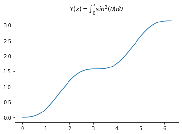
产生函数   ，并将其向量化：

In [11]:

Y_raw = lambda x: integrate(y, (theta, 0, x))
Y = np.vectorize(Y_raw)
Y

Out[11]:

<numpy.vectorize at 0xeaaff60>

In [12]:

%matplotlib inline
import matplotlib.pyplot as plt


x = np.linspace(0, 2 * np.pi)
p = plt.plot(x, Y(x))
t = plt.title(r'$Y(x) = \int_0^x sin^2(\theta) d\theta$')

数值积分

数值积分：

In [13]:

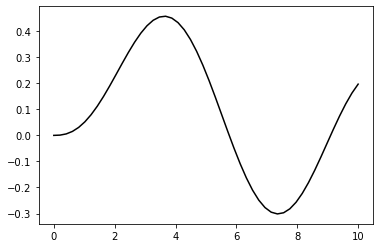
# 导入贝塞尔函数：
from scipy.special import jv


def f(x):
    return jv(2.5, x)


x = np.linspace(0, 10)
p = plt.plot(x, f(x), 'k-')

quad
 函数

Quadrature 积分的原理参见：

http://en.wikipedia.org/wiki/Numerical_integration#Quadrature_rules_based_on_interpolating_functions

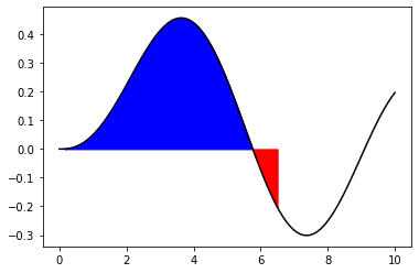
quad 返回一个 (积分值，误差) 组成的元组：

In [14]:

from scipy.integrate import quad
interval = [0, 6.5]
value, max_err = quad(f, *interval)
print("积分值：", value)
print("最大误差：", max_err)

积分值：1.2847429723410955

最大误差：2.3418185139578114e-09

积分区间图示，蓝色为正，红色为负：

In [15]:

print(f"integral = {value:.9f}")
print(f"upper bound on error: {max_err:.2e}")
x = np.linspace(0, 10, 100)
p = plt.plot(x, f(x), 'k-')
x = np.linspace(0, 6.5, 45)
p = plt.fill_between(x, f(x), where=f(x) > 0, color="blue")
p = plt.fill_between(x, f(x), where=f(x) < 0, color="red", interpolate=True)

integral = 1.284742972

upper bound on error: 2.34e-09

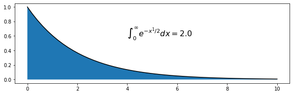
积分到无穷

In [16]:

from numpy import inf
interval = [0., inf]




def g(x):
    return np.exp(-x**1 / 2)




value, max_err = quad(g, *interval)
print(f"最大误差(upper bound on error): {max_err:.4e}")
x = np.linspace(0, 10, 50)
fig = plt.figure(figsize=(10, 3))
p = plt.plot(x, g(x), 'k-')
p = plt.fill_between(x, g(x))
plt.annotate(r"$\int_0^{\infty}e^{-x^1/2}dx = $" + str(value), (4, 0.6),
             fontsize=16)
plt.show()

最大误差(upper bound on error): 7.1615e-11

双重积分

假设我们要进行如下的积分：

  In [17]:

def h(x, t, n):
    return np.exp(-x * t) / (t ** n)

一种方式是调用两次 quad
 函数，不过这里 quad
 的返回值不能向量化，所以使用了修饰符 vectorize
 将其向量化：

In [18]:

from numpy import vectorize
@vectorize
def int_h_dx(t, n):
    """Time integrand of h(x)."""
    return quad(h, 0, np.inf, args=(t, n))[0]

In [19]:

@vectorize
def I_n(n):
    return quad(int_h_dx, 1, np.inf, args=(n))

In [20]:

I_n([0.5, 1.0, 2.0, 5])

Out[20]:

(array([2. , 1. , 0.5, 0.2]),
 array([4.507e-12, 4.340e-14, 5.551e-15, 2.220e-15]))

或者直接调用 dblquad
 函数，并将积分参数传入，传入方式有多种，后传入的先进行积分：

In [21]:

from scipy.integrate import dblquad




@vectorize
def I(n):
    """Same as I_n, but using the built-in dblquad"""
    x_lower = 0
    x_upper = np.inf
    return dblquad(h,
                   lambda t_lower: 1,
                   lambda t_upper: np.inf,
                   x_lower,
                   x_upper,
                   args=(n, ))


I_n([0.5, 1.0, 2.0, 5])

Out[21]:

(array([2. , 1. , 0.5, 0.2]),
 array([4.507e-12, 4.340e-14, 5.551e-15, 2.220e-15]))

采样点积分

trapz 方法 和 simps 方法

In [22]:

from scipy.integrate import trapz, simps


# sin 函数， 100 个采样点和 5 个采样点：
x_s = np.linspace(0, np.pi, 5)
y_s = np.sin(x_s)
x = np.linspace(0, np.pi, 100)
y = np.sin(x)


p = plt.plot(x, y, 'k:')
p = plt.plot(x_s, y_s, 'r+', markersize=12)
p = plt.fill_between(x_s, y_s, color="gray")

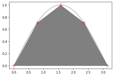
sin
 函数， 100
 个采样点和 5
 个采样点：

采用 trapezoidal 方法 和 simpson 方法 对这些采样点进行积分（函数积分为 2）：

In [23]:

print(f"trapezoidal 方法对5个采样点积分 : {trapz(y_s, x_s):.3f}")
print(f"simpson 方法对5个采样点积分 : {simps(y_s, x_s):.3f}")
print(f"trapezoidal 方法对100个采样点积分 : {trapz(y, x):.3f}")
print(f"simpson 方法对100个采样点积分 : {simps(y, x):.3f}")

trapezoidal 方法对5个采样点积分 : 1.896
simpson 方法对5个采样点积分 : 2.005
trapezoidal 方法对100个采样点积分 : 2.000
simpson 方法对100个采样点积分 : 2.000

使用 ufunc 进行积分

Numpy
 中有很多 ufunc
 对象：

In [24]:

type(np.add)

Out[24]:

numpy.ufunc

In [25]:

# np.add.accumulate 相当于 cumsum ：
np.info(np.add.accumulate)

accumulate(array, axis=0, dtype=None, out=None)

Accumulate the result of applying the operator to all elements.

For a one-dimensional array, accumulate produces results equivalent to::

  r = np.empty(len(A))
  t = op.identity        # op = the ufunc being applied to A's  elements
  for i in range(len(A)):
      t = op(t, A[i])
      r[i] = t
  return r

For example, add.accumulate() is equivalent to np.cumsum().

For a multi-dimensional array, accumulate is applied along only one
axis (axis zero by default; see Examples below) so repeated use is
necessary if one wants to accumulate over multiple axes.

Parameters
----------
array : array_like
    The array to act on.
axis : int, optional
    The axis along which to apply the accumulation; default is zero.
dtype : data-type code, optional
    The data-type used to represent the intermediate results. Defaults
    to the data-type of the output array if such is provided, or the
    the data-type of the input array if no output array is provided.
out : ndarray, None, or tuple of ndarray and None, optional
    A location into which the result is stored. If not provided or None,
    a freshly-allocated array is returned. For consistency with
    ``ufunc.__call__``, if given as a keyword, this may be wrapped in a
    1-element tuple.

    .. versionchanged:: 1.13.0
       Tuples are allowed for keyword argument.

Returns
-------
r : ndarray
    The accumulated values. If `out` was supplied, `r` is a reference to
    `out`.

Examples
--------
1-D array examples:

>>> np.add.accumulate([2, 3, 5])
array([ 2,  5, 10])
>>> np.multiply.accumulate([2, 3, 5])
array([ 2,  6, 30])

2-D array examples:

>>> I = np.eye(2)
>>> I
array([[1.,  0.],
       [0.,  1.]])

Accumulate along axis 0 (rows), down columns:

>>> np.add.accumulate(I, 0)
array([[1.,  0.],
       [1.,  1.]])
>>> np.add.accumulate(I) # no axis specified = axis zero
array([[1.,  0.],
       [1.,  1.]])

Accumulate along axis 1 (columns), through rows:

>>> np.add.accumulate(I, 1)
array([[1.,  1.],
       [0.,  1.]])

In [26]:

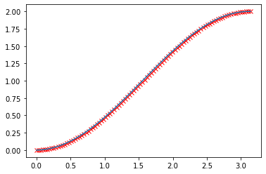
from sympy.abc import theta
y = sympy.sin(theta)
display(y)
Y = integrate(y)
display(Y)

In [27]:

x = np.linspace(0, np.pi, 100)
y = np.sin(x)
diff = x[1] - x[0]
result_np = np.add.accumulate(y) * diff
p = plt.plot(x, - np.cos(x) + np.cos(0), 'rx')
p = plt.plot(x, result_np)
print(result_np[-1])
print((- np.cos(x) + np.cos(0))[-1])

1.9998321638939924

2.0

速度比较

计算积分：

In [28]:

import sympy
from sympy.abc import x as sympy_x, theta

In [29]:

end = np.pi * 20
x = np.linspace(0, end, 10000)
y = np.sin(x)
sympy_y = vectorize(lambda x: sympy.integrate(sympy.sin(theta), (theta, 0, x)))

numpy
 方法：

In [30]:

%timeit np.add.accumulate(y) * (x[1] - x[0])
y0 = np.add.accumulate(y) * (x[1] - x[0])
print("result = ", y0[-1])

64.7 µs ± 6.37 µs per loop (mean ± std. dev. of 7 runs, 10000 loops each)

result =  -2.3413804475641734e-17

quad
 方法：

In [31]:

%timeit quad(np.sin, 0, end)
value, max_err = quad(np.sin, 0, end)
print("result = ", value)

40.6 µs ± 7.68 µs per loop (mean ± std. dev. of 7 runs, 10000 loops each)

result =  3.437813371530083e-15

trapz
 方法：

In [32]:

%timeit trapz(y, x)
y1 = trapz(y, x)
print("result = ", y1)

121 µs ± 15 µs per loop (mean ± std. dev. of 7 runs, 10000 loops each)

result =  -4.440892098500626e-16

simps
 方法：

In [33]:

%timeit simps(y, x)
y3 = simps(y, x)
print("result = ", y3)

596 µs ± 15.6 µs per loop (mean ± std. dev. of 7 runs, 1000 loops each)

result =  3.284285549683824e-16

sympy
 积分方法：

In [35]:

%timeit sympy_y(end)
y4 = sympy_y(end)
print("result = ", y4)

6.82 ms ± 789 µs per loop (mean ± std. dev. of 7 runs, 100 loops each)

result =  0