python实现曲线拟合

漫谈大数据与数据分析 2020-04-11

2261

曲线拟合

导入基础包：

In [1]:

import numpy as np
import matplotlib as mpl
import matplotlib.pyplot as plt


plt.rcParams["font.family"] = "SimHei"
plt.rcParams["axes.unicode_minus"] = False

多项式拟合

In [2]:

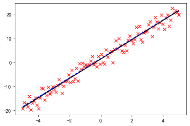
# 导入线多项式拟合工具：
from numpy import polyfit, poly1d
# 产生数据：
x = np.linspace(-5, 5, 100)
y = 4 * x + 1.5
noise_y = y + np.random.randn(y.shape[-1]) * 2.5


# 画出数据：
%matplotlib inline


p = plt.plot(x, noise_y, 'rx')
p = plt.plot(x, y, 'b:')

进行线性拟合，polyfit
是多项式拟合函数，线性拟合即一阶多项式：

In [3]:

coeff = polyfit(x, noise_y, 1)
print(coeff)

[4.01749439 1.25205778]

一阶多项式拟合，返回两个系数。

画出拟合曲线：

In [4]:

p = plt.plot(x, noise_y, 'rx')
p = plt.plot(x, y, 'b--')
p = plt.plot(x, coeff[0] * x + coeff[1], 'k-')

还可以用 poly1d
生成一个以传入的 coeff
为参数的多项式函数：

In [5]:

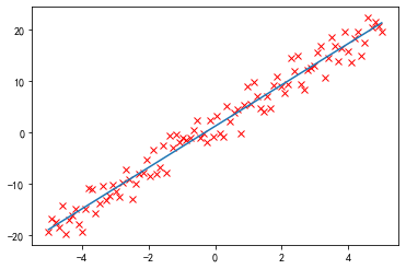
f = poly1d(coeff)
p = plt.plot(x, noise_y, 'rx')
p = plt.plot(x, f(x))

In [6]:

display(f)
print(f)
poly1d([4.01749439, 1.25205778])

 
4.017 x + 1.252

还可以对它进行数学操作生成新的多项式：

In [7]:

print(f + 2 * f ** 2)

       2
32.28 x + 24.14 x + 4.387

多项式拟合正弦函数

正弦函数：

In [8]:

x = np.linspace(-np.pi, np.pi, 100)
y = np.sin(x)

用一阶到九阶多项式拟合，类似泰勒展开：

In [9]:

y1 = poly1d(polyfit(x, y, 1))
y3 = poly1d(polyfit(x, y, 3))
y5 = poly1d(polyfit(x, y, 5))
y7 = poly1d(polyfit(x, y, 7))
y9 = poly1d(polyfit(x, y, 9))

In [10]:

x = np.linspace(-3 * np.pi, 3 * np.pi, 300)


p = plt.plot(x, np.sin(x), 'k', label="sin(x)")
p = plt.plot(x, y1(x), label="1")
p = plt.plot(x, y3(x), label="3")
p = plt.plot(x, y5(x), label="5")
p = plt.plot(x, y7(x), label="7")
p = plt.plot(x, y9(x), label="9")


a = plt.axis([-3 * np.pi, 3 * np.pi, -1.25, 1.25])
plt.legend()
plt.show()

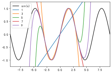
黑色为原始的图形，可以看到，随着多项式拟合的阶数的增加，曲线与拟合数据的吻合程度在逐渐增大。

最小二乘拟合

导入相关的模块：

In [11]:

from scipy.linalg import lstsq
from scipy.stats import linregress

In [12]:

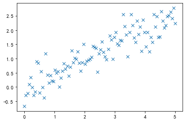
x = np.linspace(0, 5, 100)
y = 0.5 * x + np.random.randn(x.shape[-1]) * 0.35


plt.plot(x, y, 'x')

Out[12]:

[<matplotlib.lines.Line2D at 0x17582ef0>]

Scipy.linalg.lstsq 最小二乘解

一般，当使用一个 N-1 阶的多项式拟合这 M 个点时，有这样的关系存在：

即

要得到 C
，可以使用 scipy.linalg.lstsq
求最小二乘解。

这里，我们使用 1 阶多项式即 N = 2
，先将 x
扩展成 X
：

In [13]:

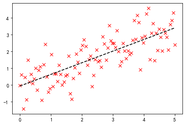
x = np.linspace(0, 5, 100)
h = np.random.randn(x.shape[-1]) * 0.8
y = 0.7 * x + h
print(f"原函数f(x)=0.7x+0.8*N(0,1)")
X = np.hstack((x[:, np.newaxis], np.ones((x.shape[-1], 1))))
# 求解：
C, resid, rank, s = lstsq(X, y)
print(f"拟合函数f(x)={C[0]}x+{C[1]}")
print(f"残差平方和(sum squared residual) = {resid:.3f}")
print(f"矩阵X的秩(rank of the X matrix) = {rank}")
print(f"奇异值分解(singular values of X) = {s}")
# 画图：
p = plt.plot(x, y, 'rx')
p = plt.plot(x, C[0] * x + C[1], 'k--')

原函数f(x)=0.7x+0.8*N(0,1)
拟合函数f(x)=0.6934440249789187x+-0.05730421805802857
残差平方和(sum squared residual) = 70.446
矩阵X的秩(rank of the X matrix) = 2
奇异值分解(singular values of X) = [30.23732043  4.82146667]

Scipy.stats.linregress 线性回归

In [14]:

slope, intercept, r_value, p_value, stderr = linregress(x, y)
print("原函数f(x)=0.7x+0.8*N(0,1)")
print(f"拟合函数f(x)={slope}x+{intercept}")
print(f"R-value = {r_value:.3f}")
print(f"p-value (probability there is no correlation) = {p_value:.3e}")
print(f"均方误差RMSE(Root mean squared error of the fit) = {np.sqrt(stderr):.3f}")


p = plt.plot(x, y, 'rx')
p = plt.plot(x, slope * x + intercept, 'k--')

原函数f(x)=0.7x+0.8*N(0,1)
拟合函数f(x)=0.6934440249789185x+-0.05730421805802832
R-value = 0.769
p-value (probability there is no correlation) = 8.710e-21
均方误差RMSE(Root mean squared error of the fit) = 0.241

可以看到，两者求解的结果是一致的，但是出发的角度是不同的。

更高级的拟合

定义非线性函数：

In [15]:

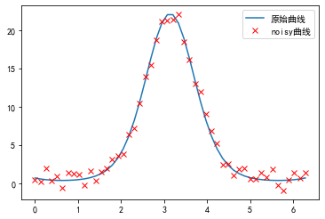
def function(x, a , b, f, phi):
    result = a * np.exp(-b * np.sin(f * x + phi))
    return result


In [16]:from scipy.optimize import leastsq


x = np.linspace(0, 2 * np.pi, 50)
actual_parameters = [3, 2, 1.25, np.pi / 4]
y = function(x, *actual_parameters)
# 画出原始曲线：
p = plt.plot(x, y, label="原始曲线")


# 加入噪声：
from scipy.stats import norm
y_noisy = y + 0.9 * norm.rvs(size=len(x))
p = plt.plot(x, y_noisy, 'rx', label="noisy曲线")


plt.legend()

Out[16]:

<matplotlib.legend.Legend at 0x175aecf8>

Scipy.optimize.leastsq

定义误差函数，将要优化的参数放在前面：

In [17]:

def f_err(p, y, x):
    return y - function(x, *p)

将这个函数作为参数传入 leastsq
函数，第二个参数为初始值：

In [18]:

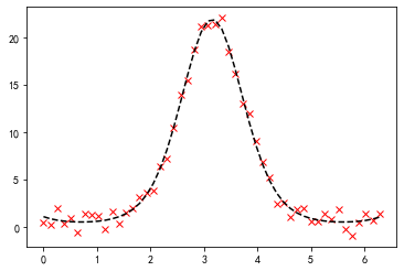
c, ret_val = leastsq(f_err, [1, 1, 1, 1], args=(y_noisy, x))
c, ret_val

Out[18]:

(array([3.44391769, 1.85133714, 1.28397522, 0.66189323]), 1)

ret_val
是 1~4 时，表示成功找到最小二乘解：

In [19]:

p = plt.plot(x, y_noisy, 'rx')
p = plt.plot(x, function(x, *c), 'k--')

Scipy.optimize.curve_fit

更高级的做法：

In [20]:

from scipy.optimize import curve_fit
# 不需要定义误差函数，直接传入 function 作为参数：
p_est, err_est = curve_fit(function, x, y_noisy)
# 函数的参数
print("函数的参数:", p_est)
print("协方差矩阵:\n", err_est)
p = plt.plot(x, y_noisy, "rx")
p = plt.plot(x, function(x, *p_est), "k--")

函数的参数: [3.44391759 1.85133717 1.2839752  0.66189328]
协方差矩阵:
 [[ 0.08298696 -0.02387346  0.00890623 -0.02808425]
 [-0.02387346  0.00706822 -0.0024504   0.00772683]
 [ 0.00890623 -0.0024504   0.00132793 -0.00418765]
 [-0.02808425  0.00772683 -0.00418765  0.01336865]]

协方差矩阵的对角线为各个参数的方差：

In [21]:

print("协方差矩阵的对角线为各个参数的方差(normalized relative errors for each parameter)：")
print("   a\t  b\t f\tphi")
print(np.sqrt(err_est.diagonal()) / p_est)

协方差矩阵的对角线为各个参数的方差(normalized relative errors for each parameter)：
   a	  b	 f	phi
[0.08364735 0.0454119  0.02838125 0.1746851 ]

python

文章转载自漫谈大数据与数据分析，如果涉嫌侵权，请发送邮件至：contact@modb.pro进行举报，并提供相关证据，一经查实，墨天轮将立刻删除相关内容。