R语言可视化（十八）：UMAP图绘制

bioinfomics 2020-10-05

1827

18. UMAP图绘制

清除当前环境中的变量

rm(list=ls())

设置工作目录

setwd("C:/Users/Dell/Desktop/R_Plots/18umap/")

查看示例数据

head(iris)
##   Sepal.Length Sepal.Width Petal.Length Petal.Width Species
## 1          5.1         3.5          1.4         0.2  setosa
## 2          4.9         3.0          1.4         0.2  setosa
## 3          4.7         3.2          1.3         0.2  setosa
## 4          4.6         3.1          1.5         0.2  setosa
## 5          5.0         3.6          1.4         0.2  setosa
## 6          5.4         3.9          1.7         0.4  setosa

iris.data = iris[,c(1:4)]
iris.labels = iris$Species
head(iris.data)
##   Sepal.Length Sepal.Width Petal.Length Petal.Width
## 1          5.1         3.5          1.4         0.2
## 2          4.9         3.0          1.4         0.2
## 3          4.7         3.2          1.3         0.2
## 4          4.6         3.1          1.5         0.2
## 5          5.0         3.6          1.4         0.2
## 6          5.4         3.9          1.7         0.4

head(iris.labels)
## [1] setosa setosa setosa setosa setosa setosa
## Levels: setosa versicolor virginica

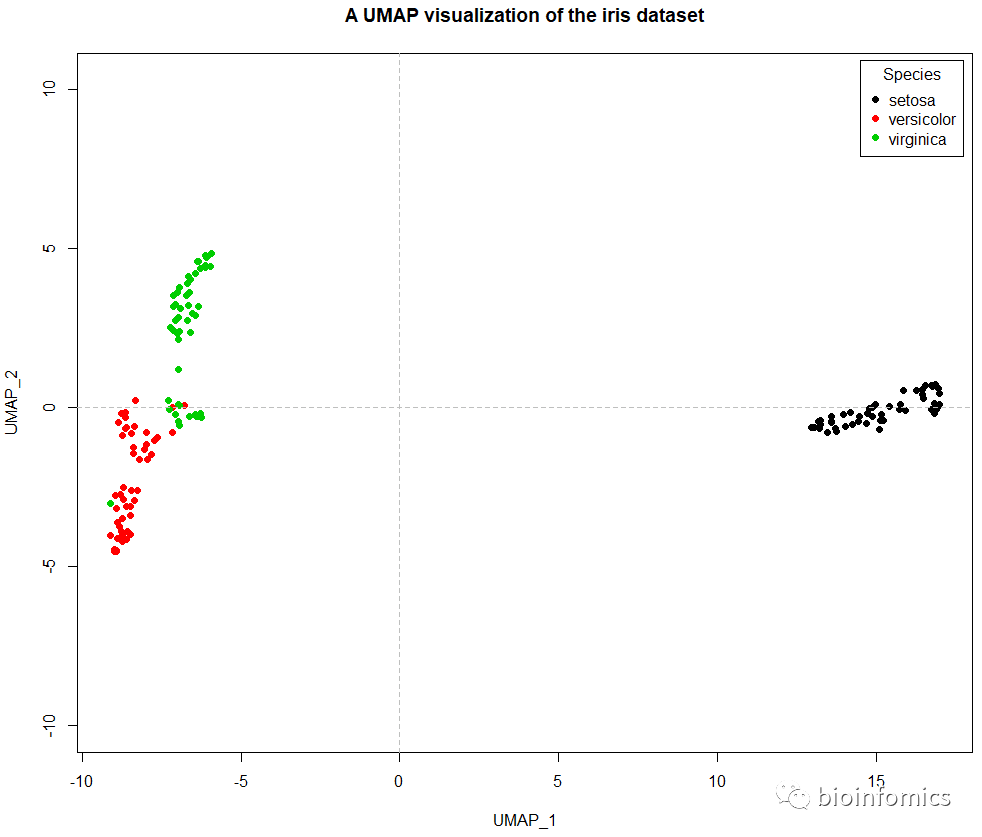
使用umap包进行UMAP降维可视化分析

library(umap)

# 使用umap函数进行UMAP降维分析
iris.umap = umap::umap(iris.data)
iris.umap
## umap embedding of 150 items in 2 dimensions
## object components: layout, data, knn, config

# 查看降维后的结果
head(iris.umap$layout)
##          [,1]     [,2]
## [1,] 12.59949 3.759360
## [2,] 13.80894 5.272737
## [3,] 14.43500 4.813293
## [4,] 14.36174 4.896541
## [5,] 12.80543 3.473356
## [6,] 12.14902 2.715970

# 使用plot函数可视化UMAP的结果
plot(iris.umap$layout,col=iris.labels,pch=16,asp = 1,
     xlab = "UMAP_1",ylab = "UMAP_2",
     main = "A UMAP visualization of the iris dataset")
# 添加分隔线
abline(h=0,v=0,lty=2,col="gray")
# 添加图例
legend("topright",title = "Species",inset = 0.01,
       legend = unique(iris.labels),pch=16,
       col = unique(iris.labels))

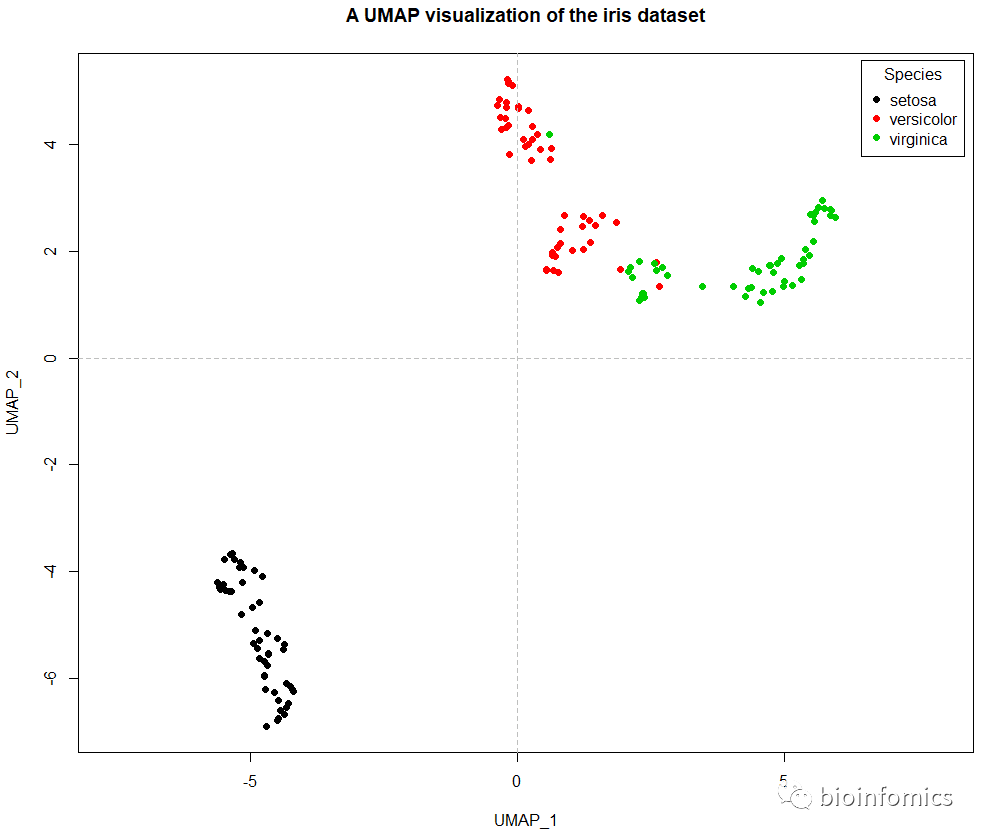
使用uwot包进行UMAP降维可视化分析

library(uwot)

head(iris)
##   Sepal.Length Sepal.Width Petal.Length Petal.Width Species
## 1          5.1         3.5          1.4         0.2  setosa
## 2          4.9         3.0          1.4         0.2  setosa
## 3          4.7         3.2          1.3         0.2  setosa
## 4          4.6         3.1          1.5         0.2  setosa
## 5          5.0         3.6          1.4         0.2  setosa
## 6          5.4         3.9          1.7         0.4  setosa

# 使用umap函数进行UMAP降维分析
iris_umap <- uwot::umap(iris)
head(iris_umap)
##            [,1]      [,2]
## [1,] -10.009518 -4.084256
## [2,]  -9.505712 -5.754688
## [3,] -10.056058 -5.995699
## [4,]  -9.884181 -6.000248
## [5,] -10.066767 -4.143123
## [6,] -10.620676 -3.369200

# 使用plot函数可视化UMAP降维的结果
plot(iris_umap,col=iris$Species,pch=16,asp = 1,
     xlab = "UMAP_1",ylab = "UMAP_2",
     main = "A UMAP visualization of the iris dataset")
# 添加分隔线
abline(h=0,v=0,lty=2,col="gray")
# 添加图例
legend("topright",title = "Species",inset = 0.01,
       legend = unique(iris$Species),pch=16,
       col = unique(iris$Species))

# Supervised dimension reduction using the 'Species' factor column
iris_sumap <- uwot::umap(iris, n_neighbors = 15, min_dist = 0.001,
                   y = iris$Species, target_weight = 0.5)
head(iris_sumap)
##           [,1]      [,2]
## [1,] -10.79467 -14.11691
## [2,] -11.99333 -13.15741
## [3,] -12.39469 -13.71514
## [4,] -12.54123 -13.47225
## [5,] -10.89463 -14.27025
## [6,] -10.15880 -13.58669

iris_sumap_res <- data.frame(iris_sumap,Species=iris$Species)
head(iris_sumap_res)
##          X1        X2 Species
## 1 -10.79467 -14.11691  setosa
## 2 -11.99333 -13.15741  setosa
## 3 -12.39469 -13.71514  setosa
## 4 -12.54123 -13.47225  setosa
## 5 -10.89463 -14.27025  setosa
## 6 -10.15880 -13.58669  setosa

# 使用ggplot2包可视化UMAP降维的结果
library(ggplot2)

ggplot(iris_sumap_res,aes(X1,X2,color=Species)) + 
  geom_point() + theme_bw() + 
  geom_hline(yintercept = 0,lty=2,col="red") + 
  geom_vline(xintercept = 0,lty=2,col="blue",lwd=1) +
  theme(plot.title = element_text(hjust = 0.5)) + 
  labs(x="UMAP_1",y="UMAP_2",
       title = "A UMAP visualization of the iris dataset")

sessionInfo()
## R version 3.6.0 (2019-04-26)
## Platform: x86_64-w64-mingw32/x64 (64-bit)
## Running under: Windows 10 x64 (build 18363)
##
## Matrix products: default
##
## locale:
## [1] LC_COLLATE=Chinese (Simplified)_China.936
## [2] LC_CTYPE=Chinese (Simplified)_China.936
## [3] LC_MONETARY=Chinese (Simplified)_China.936
## [4] LC_NUMERIC=C
## [5] LC_TIME=Chinese (Simplified)_China.936
##
## attached base packages:
## [1] stats     graphics  grDevices utils     datasets  methods   base
##
## other attached packages:
## [1] ggplot2_3.2.0 uwot_0.1.4    Matrix_1.2-17 umap_0.2.6.0
##
## loaded via a namespace (and not attached):
##  [1] Rcpp_1.0.5         RSpectra_0.15-0    compiler_3.6.0
##  [4] pillar_1.4.2       tools_3.6.0        digest_0.6.20
##  [7] jsonlite_1.6       evaluate_0.14      tibble_2.1.3
## [10] gtable_0.3.0       lattice_0.20-38    pkgconfig_2.0.2
## [13] rlang_0.4.7        yaml_2.2.0         xfun_0.8
## [16] withr_2.1.2        stringr_1.4.0      dplyr_0.8.3
## [19] knitr_1.23         askpass_1.1        tidyselect_0.2.5
## [22] grid_3.6.0         glue_1.3.1         reticulate_1.13
## [25] R6_2.4.0           rmarkdown_1.13     purrr_0.3.2
## [28] magrittr_1.5       scales_1.0.0       htmltools_0.3.6
## [31] assertthat_0.2.1   colorspace_1.4-1   labeling_0.3
## [34] stringi_1.4.3      RcppParallel_4.4.4 openssl_1.4
## [37] lazyeval_0.2.2     munsell_0.5.0      crayon_1.3.4
## [40] FNN_1.1.3