


CS261: A Second Course in Algorithms
Lecture #1: Course Goals and Introduction to
Maximum Flow∗
Tim Roughgarden†
January 5, 2016
1
Course Goals
CS261 has two major course goals, and the courses splits roughly in half along these lines.
1
.1 Well-Solved Problems
This first goal is very much in the spirit of an introductory course on algorithms. Indeed,
the first few weeks of CS261 are pretty much a direct continuation of CS161 — the topics
that we’d cover at the end of CS161 at a semester school.
Course Goal 1 Learn efficient algorithms for fundamental and well-solved problems.
There’s a collection of problems that are flexible enough to model many applications and
can also be solved quickly and exactly, in both theory and practice. For example, in CS161
you studied shortest-path algorithms. You should have learned all of the following:
1
2
. The formal definition of one or more variants of the shortest-path problem.
. Some famous shortest-path algorithms, like Dijkstra’s algorithm and the Bellman-Ford
algorithm, which belong in the canon of algorithms’ greatest hits.
3
. Applications of shortest-path algorithms, including to problems that don’t explicitly
involve paths in a network. For example, to the problem of planning a sequence of
decisions over time.
∗
†
ꢀc
2
Department of Computer Science, Stanford University, 474 Gates Building, 353 Serra Mall, Stanford,
016, Tim Roughgarden.
CA 94305. Email: tim@cs.stanford.edu.
1

The study of such problems is top priority in a course like CS161 or CS261. One of
the biggest benefits of these courses is that they prevent you from reinventing the wheel
(or trying to invent something that doesn’t exist), instead allowing you to stand on the
shoulders of the many brilliant computer scientists who preceded us. When you encounter
such problems, you already have good algorithms in your toolbox and don’t have to design
one from scratch. This course will also give you practice spotting applications that are just
thinly disguised versions of these problems.
Specifically, in the first half of the course we’ll study:
1
2
3
4
. the maximum flow problem;
. the minimum cut problem;
. graph matching problems;
. linear programming, one the most general polynomial-time solvable problems known.
Our algorithms for these problems with have running times a bit bigger than those you
studied in CS161 (where almost everything runs in near-linear time). Still, these algorithms
are sufficiently fast that you should be happy if a problem that you care about reduces to
one of these problems.
1
.2 Not-So-Well-Solved Problems
Course Goal 2 Learns tools for tackling not-so-well-solved problems.
Unfortunately, many real-world problems fall into this camp, for many different reasons.
We’ll focus on two classes of such problems.
1
. NP-hard problems, for which we don’t expect there to be any exact polynomial-time
algorithms. We’ll study several broadly useful techniques for designing and analyzing
heuristics for such problems.
2
. Online problems. The anachronistic name does not refer to the Internet or social
networks, but rather to the realistic case where an algorithm must make irrevocable
decisions without knowing the future (i.e., without knowing the whole input).
We’ll focus on algorithms for NP-hard and online problems that are guaranteed to output
a solution reasonably close to an optimal one.
1
.3 Intended Audience
CS261 has two audiences, both important. The first is students who are taking their final
algorithms course. For this group, the goal is to pack the course with essential and likely-
to-be-useful material. The second is students who are contemplating a deeper study of
algorithms. With this group in mind, when the opportunity presents itself, we’ll discuss
2
recent research developments and give you a glimpse of what you’ll see in future algorithms
courses. For this second audience, CS261 has a third goal.
Course Goal 3 Provide a gateway to the study of advanced algorithms.
After completing CS261, you’ll be well equipped to take any of the many 200- and 300-
level algorithms courses that the department offers. The pace and difficulty level of CS261
interpolates between that of CS161 and more advanced theory courses.
When you speak to audience, it’s good to have one or a few “canonical audience members”
in mind. For your reference and amusement, here’s your instructor’s mental model for
canonical students in courses at different levels:
1
2
. CS161: a constant fraction of the students do not want to be there, and/or hate math.
. CS261: a self-selecting group of students who like algorithms and want to learn much
more about them. Students may or may not love math, but they shouldn’t hate it.
3
. CS3xx: geared toward students who are doing or would like to do research in algo-
rithms.
2
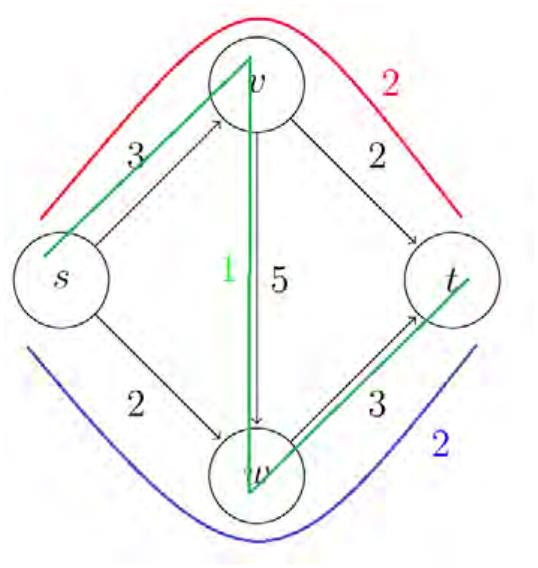
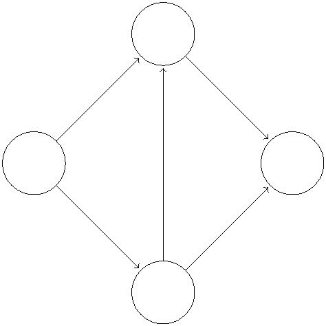
Introduction to the Maximum Flow Problem
v
3
2
2
3
s
5
t
w
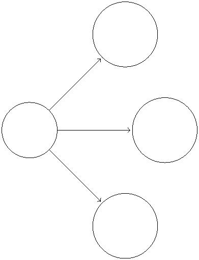
Figure 1: (a, left) Our first flow network. Each edge is associated with a capacity. (b, right)
A sample flow of value 5, where the red, green and blue paths have flow values of 2, 1, 2
respectively.
2
.1 Problem Definition
The maximum flow problem is a stone-cold classic in the design and analysis of algorithms.
It’s easy to understand intuitively, so let’s do an informal example before giving the formal
3

definition.
The picture in Figure 1(a) resembles the ones you saw when studying shortest paths, but
the semantics are different. Each edge is labeled with a capacity, the maximum amount of
stuff that it can carry. The goal is to figure out how much stuff can be pushed from the
vertex s to the vertex t.
For example, Figure 1(b) exhibits a method of pushing five units of flow from s to t, while
respecting all edges’ capacities. Can we do better? Certainly not, since at most 5 units of
flow can escape s on its two outgoing edges.
Formally, an instance of the maximum flow problem is specified by the following ingre-
dients:
•
•
•
•
a directed graph G, with vertices V and directed edges E;1
a source vertex s ∈ V ;
a sink vertex t ∈ V ;
a nonnegative and integral capacity ue for each edge e ∈ E.
v
3
(3)
(2)
2 (2)
s
5 (1)
t
2
3 (3)
w
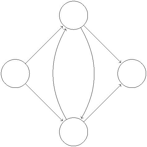
Figure 2: Denoting a flow by keeping track of the amount of flow on each edge. Flow amount
is given in brackets.
.
Since the point is to push flow from s to t, we can assume without loss of generality
that s has no incoming edges and t has no outgoing edges.
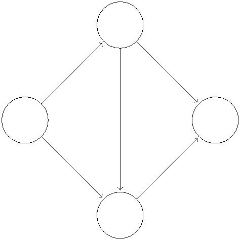
Given such an input, the feasible solutions are the flows in the network. While Figure 1(b)
depicts a flow in terms of several paths, for algorithms, it works better to just keep track of
the amount of flow on each edge (as in Figure 2).2 Formally, a flow is a nonnegative vector
{
fe}e∈E, indexed by the edges of G, that satisfies two constraints:
1
All of our maximum flow algorithms can be extended to undirected graphs; see Exercise Set #1.
Every flow in this sense arises as the superposition of flow paths and flow cycles; see Problem #1.
2
4

Capacity constraints: f ≤ u for every edge e ∈ E;
e
e
Conservation constraints: for every vertex v other than s and t,
amount of flow entering v = amount of flow exiting v.
The left-hand side is the sum of the fe’s over the edge incoming to v; likewise with the
outgoing edges for the right-hand side.
The objective is to compute a maximum flow — a flow with the maximum-possible value,
meaning the total amount of flow that leaves s. (As we’ll see, this is the same as the total
amount of flow that enters t.)
2
.2 Applications
Why should we care about the maximum flow problem? Like all central algorithmic prob-
lems, the maximum flow problem is useful in its own right, plus many different problems are
really just thinly disguised version of maximum flow. For some relatively obvious and literal
applications, the maximum flow problem can model the routing of traffic through a trans-
portation network, packets through a data network, or oil through a distribution network.3
In upcoming lectures we’ll prove the less obvious fact that problems ranging from bipartite
matching to image segmentation reduce to the maximum flow problem.
2
.3 A Naive Greedy Algorithm
We now turn our attention to the design of efficient algorithms for the maximum flow prob-
lem. A priori, it is not clear that any such algorithms exist (for all we know right now, the
problem is NP-hard).
We begin by considering greedy algorithms. Recall that a greedy algorithm is one that
makes a sequence of myopic and irrevocable decisions, with the hope that everything some-
how works out at the end. For most problems, greedy algorithms do not generally produce
the best-possible solution. But it’s still worth trying them, because the ways in which greedy
algorithms break often yields insights that lead to better algorithms.
The simplest greedy approach to the maximum flow problem is to start with the all-zero
flow and greedily produce flows with ever-higher value. The natural way to proceed from
one to the next is to send more flow on some path from s to t (cf., Figure 1(b)).
3
A flow corresponds to a steady-state solution, with a constant rate of arrivals at s and departures at t.
The model does not capture the time at which flow reaches different vertices. However, it’s not hard to
extend the model to also capture temporal aspects as well.
5

A Naive Greedy Algorithm
initialize f = 0 for all e ∈ E
e
repeat
search for an s-t path P such that f < u for every e ∈ P
e
e
/
/ takes O(|E|) time using BFS or DFS
if no such path then
halt with current flow {fe}e∈E
else
room on e
z }| {
room on P
let ∆ = min (u − f )
e
e
e∈P
|
{z
}
for all edges e of P do
increase fe by ∆
Note that the path search just needs determine whether or not there is an s-t path in
the subgraph of edges e with f < u . This is easily done in linear time using your favorite
e
e
graph search subroutine, such as breadth-first or depth-first search. There may be many
such paths; for now, we allow the algorithm to choose one arbitrarily. The algorithm then
pushes as much flow as possible on this path, subject to capacity constraints.
v
3
(3)
2
s
5 (3)
t
2
3 (3)
w
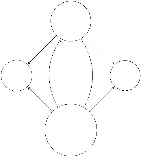
Figure 3: Greedy algorithm returns suboptimal result if first path picked is s-v-w-t.
This greedy algorithm is natural enough, but it does it work? That is, when it terminates
with a flow, need this flow be a maximum flow? Our sole example thus far already provides
a negative answer (Figure 3). Initially, with the all-zero flow, all s-t paths are fair game. If
the algorithm happens to pick the zig-zag path, then ∆ = min{3, 5, 3} = 3 and it routes 3
units of flow along the path. This saturates the upper-left and lower-right edges, at which
point there is no s-t path such that f < u on every edge. The algorithm terminates at this
e
e
6


point with a flow with value 3. We already know that the maximum flow value is 5, and we
conclude that the naive greedy algorithm can terminate with a non-maximum flow.4
2
.4 Residual Graphs
The second idea is to extend the naive greedy algorithm by allowing “undo” operations. For
example, from the point where this algorithm gets stuck in Figure 3, we’d like to route two
more units of flow along the edge (s, w), then backward along the edge (v, w), undoing 2 of
the 3 units we routed the previous iteration, and finally along the edge (v, t). This would
yield the maximum flow of Figure 1(b).
ue − fe
v
w
u (f )
e
e
v
w
fe
Figure 4: (a) original edge capacity and flow and (b) resultant edges in residual network.
v
3
2
2
3
s
2
3
t
w
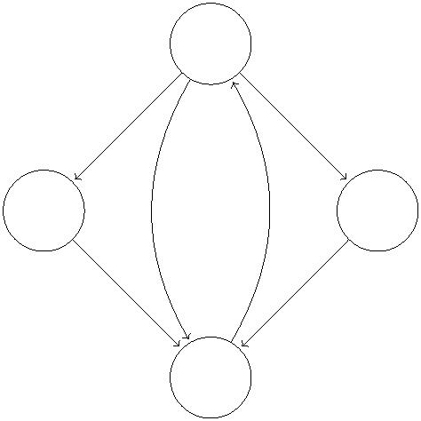
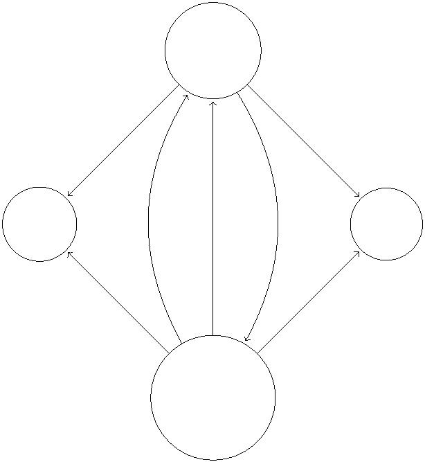
Figure 5: Residual network of flow in Figure 3.
We need a way of formally specifying the allowable “undo” operations. This motivates
the following simple but important definition, of a residual network. The idea is that, given
a graph G and a flow f in it, we form a new flow network Gf that has the same vertex set
of G and that has two edges for each edge of G. An edge e = (v, w) of G that carries flow fe
and has capacity u (Figure 4(a)) spawns a “forward edge” (u, v) of G with capacity u −f
e
f
e
e
(the room remaining) and a “backward edge” (w, v) of G with capacity f (the amount
f
e
4
It does compute what’s known as a “blocking flow;” more on this next lecture.
7


of previously routed flow that can be undone). See Figure 4(b).5 Observe that s-t paths
with f < u for all edges, as searched for by the naive greedy algorithm, correspond to the
e
e
special case of s-t paths of Gf that comprise only forward edges.
For example, with G our running example and f the flow in Figure 3, the corresponding
residual network G is shown in Figure 5. The four edges with zero capacity in G are
f
f
omitted from the picture.6
2
.5 The Ford-Fulkerson Algorithm
Happily, if we just run the natural greedy algorithm in the current residual network, we get
a correct algorithm, the Ford-Fulkerson algorithm.7
Ford-Fulkerson Algorithm
initialize f = 0 for all e ∈ E
e
repeat
search for an s-t path P in the current residual graph Gf such that
every edge of P has positive residual capacity
/
/ takes O(|E|) time using BFS or DFS
if no such path then
halt with current flow {fe}e∈E
else
let ∆ = min
/
(e’s residual capacity in Gf )
/ augment the flow f using the path P
e∈P
for all edges e of G whose corresponding forward edge is in P do
increase fe by ∆
for all edges e of G whose corresponding reverse edge is in P do
decrease fe by ∆
For example, starting from the residual network of Figure 5, the Ford-Fulkerson algorithm
will augment the flow by units along the path s → w → v → t. This augmentation produces
the maximum flow of Figure 1(b).
We now turn our attention to the correctness of the Ford-Fulkerson algorithm. We’ll
worry about optimizing the running time in future lectures.
5
If G already has two edges (v, w) and (w, v) that go in opposite directions between the same two vertices,
then Gf will have two parallel edges going in either direction. This is not a problem for any of the algorithms
that we discuss.
6
More generally, when we speak about “the residual graph,” we usually mean after all edges with zero
residual capacity have been removed.
7
Yes, it’s the same Ford from the Bellman-Ford algorithm.
8


2
.6 Termination
We claim that the Ford-Fulkerson algorithm eventually terminates with a feasible flow. This
follows from two invariants, both proved by induction on the number of iterations.
First, the algorithm maintains the invariant that {f }
is a flow. This is clearly true
initially. The parameter ∆ is defined so that no flow value f becomes negative or exceeds
e
e∈E
e
the capacity ue. For the conservation constraints, consider a vertex v. If v is not on the
augmenting path P in Gf , then the flow into and out of v remain the same. If v is on P,
with edges (x, v) and (v, w) belonging to P, then there are four cases, depending on whether
or not (x, v) and (v, w) correspond to forward or reverse edges. For example, if both are
forward edges, then the flow augmentation increases both the flow into and the flow out of
v increase by ∆. If both are reverse edges, then both the flow into and the flow out of v
decrease by ∆. In all four cases, the flow in and flow out change by the same amount, so
conservation constraints are preserved.
Second, the Ford-Fulkerson algorithm maintains the property that every flow amount fe
is an integer. (Recall we are assuming that every edge capacity ue is an integer.) Inductively,
all residual capacities are integral, so the parameter ∆ is integral, so the flow stays integral.
Every iteration of the Ford-Fulkerson algorithm increase the value of the current flow by
the current value of ∆. The second invariant implies that ∆ ≥ 1 in every iteration of the
Ford-Fulkerson algorithm. Since only a finite amount of flow can escape the source vertex,
the Ford-Fulkerson algorithm eventually halts. By the first invariant, it halts with a feasible
flow.8
Of course, all of this applies equally well to the naive greedy algorithm of Section 2.3.
How do we know whether or not the Ford-Fulkersonalgorithm can also terminate with a non-
maximum flow? The hope is that because the Ford-Fulkersonalgorithm has more path eligible
for augmentation, it progresses further before halting. But is it guaranteed to compute a
maximum flow?
2
.7 Optimality Conditions
Answering the following question will be a major theme of the first half of CS261, culminating
with our study of linear programming duality.
HOW DO WE KNOW WHEN WE’RE DONE?
For example, given a flow, how do we know if it’s a maximum flow? Any correct maximum
flow algorithm must answer this question, explicitly or implicitly. If I handed you an allegedly
maximum flow, how could I convince you that I’m not lying? It’s easy to convince someone
that a flow is not maximum, just by exhibiting a flow with higher value.
8
The Ford-Fulkersonalgorithm continues to terminate if edges’ capacities are rational numbers, not nec-
essarily integers. (Proof: scaling all capacities by a common number doesn’t change the problem, so we can
clear denominators to reduce the rational capacity case to the integral capacity case.) It is a bizarre mathe-
matical curiosity that the Ford-Fulkersonalgorithm need not terminate with edges’ capacities are irrational.
9

Returning to our original example (Figure 1), answering this question didn’t seem like a
big deal. We exhibited a flow of value 5, and because the total capacity escaping s is only 5,
it’s clear that there can’t be any flow with high value. But what about the network in
Figure 6(a)? The flow shown in Figure 6(b) has value only 3. Could it really be a maximum
flow?
v
v
1
(1)
100 (2)
t
1
100
s
1
t
s
1 (1)
1
00
1
100 (2)
1 (1)
w
w
Figure 6: (a) A given network and (b) the alleged maximum flow of value 3.
We’ll tackle several fundamental computational problems by following a two-step paradigm.
Two-Step Paradigm
1
2
. Identify “optimality conditions” for the problem. These are sufficient
conditions for a feasible solution to be an optimal solution. This step is
structural, and not necessarily algorithmic. The optimality conditions
vary with the problem, but they are often quite intuitive.
. Design an algorithm that terminates with the optimality conditions sat-
isfied. Such an algorithm is necessarily correct.
This paradigm is a guide for proving algorithms correct. Correctness proofs didn’t get too
much airtime in CS161, because almost all of them are straightforward inductions — think
of MergeSort, or Dijkstra’s algorithm, or any dynamic programming algorithm. The harder
problems studied in CS261 demand a more sophisticated and principle approach (with which
you’ll get plenty of practice).
So how would we apply this two-step paradigm to the maximum flow problem? Consider
the following claim.
Claim 2.1 (Optimality Conditions for Maximum Flow) If f is a flow in G such that
the residual network Gf has no s-t path, then the f is a maximum flow.
1
0


This claim implements the first step of the paradigm. The Ford-Fulkersonalgorithm, which
can only terminate with this optimality condition satisfied, already provides a solution to
the second step. We conclude:
Corollary 2.2 The Ford-Fulkersonalgorithm is guaranteed to terminate with a maximum
flow.
Next lecture we’ll prove (a generalization of) the claim, derive the famous maximum-
flow/minimum-cut problem, and design faster maximum flow algorithms.
1
1
CS261: A Second Course in Algorithms
Lecture #2: Augmenting Path Algorithms for
Maximum Flow∗
Tim Roughgarden†
January 7, 2016
1
Recap
ue − fe
v
w
u (f )
e
e
v
w
fe
Figure 1: (a) original edge capacity and flow and (b) resultant edges in residual network.
Recall where we left off last lecture. We’re considering a directed graph G = (V, E) with a
source s, sink t, and an integer capacity u for each edge e ∈ E. A flow is a nonnegative vector
e
{
f }
that satisfies capacity constraints (f ≤ u for all e) and conservation constraints
e
(flow in = flow out except at s and t).
e∈E
e
e
Recall that given a flow f in a graph G, the corresponding residual network has two edges
for each edge e of G, a forward edge with residual capacity u − f and a reverse edge with
e
e
residual capacity f that allows us to “undo” previously routed flow. See also Figure 1.1
e
The Ford-Fulkerson algorithm repeatedly finds an s-t path P in the current residual
graph Gf , and augments along p as much as possible subject to the capacity constraints of
∗
†
ꢀc
2
Department of Computer Science, Stanford University, 474 Gates Building, 353 Serra Mall, Stanford,
016, Tim Roughgarden.
CA 94305. Email: tim@cs.stanford.edu.
We usually implicitly assume that all edges with zero residual capacity are omitted from the residual
network.
1
1

the residual network.2 We argued that the algorithm eventually terminates with a feasible
flow. But is it a maximum flow? More generally, a major course theme is to understand
How do we know when we’re done?
For example, could the maximum flow value in the network in Figure 2 really just be 3?
v
v
1
(1)
100 (2)
t
1
100
s
1
t
s
1 (1)
1
00
1
100 (2)
1 (1)
w
w
Figure 2: (a) A given network and (b) the alleged maximum flow of value 3.
2
Around the Maximum-Flow/Minimum-Cut Theorem
We ended last lecture with a claim that if there is no s-t path (with positive residual ca-
pacity on every edge) in the residual graph Gf , then f is a maximum flow in G. It’s conve-
nient to prove a stronger statement, from which we can also derive the famous maximum-
flow/minimum cut theorem.
2
.1 (s, t)-Cuts
To state the stronger result, we need an important definition, of objects that are “dual” to
flows in a sense we’ll make precise later.
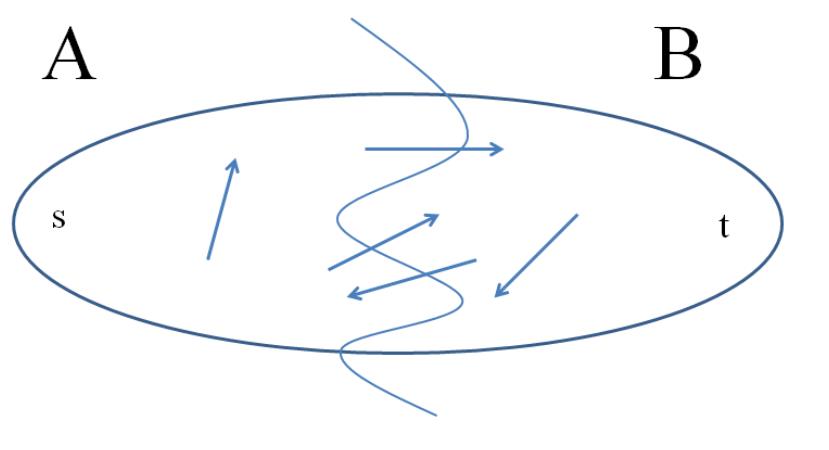
Definition 2.1 (s-t Cut) An (s, t)-cut of a graph G = (V, E) is a partition of V into sets
A, B with s ∈ A and t ∈ B.
Sometimes we’ll simply say “cut” instead of “(s, t)-cut.”
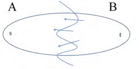
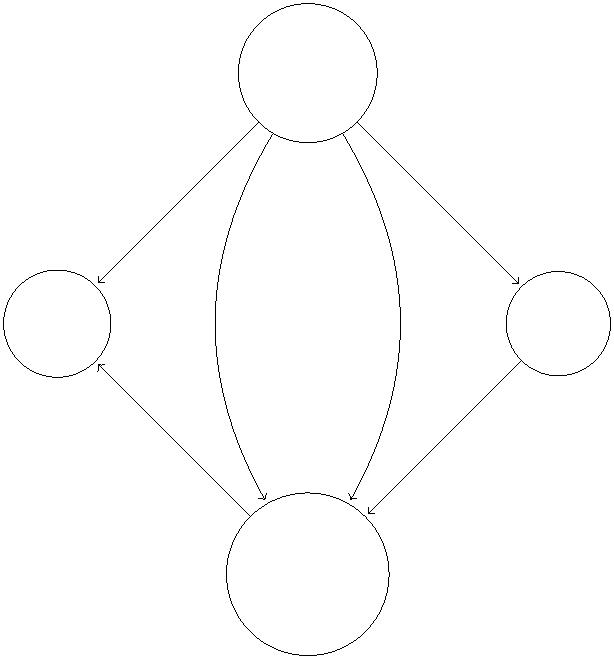
Figure 3 depicts a good (if cartoonish) way to think about an (s, t)-cut of a graph. Such
a cut buckets the edges of the graph into four categories: those with both endpoints in A,
those with both endpoints in B, those sticking out of A (with tail in A and head in B), and
those sticking into A (with head in A and tail in B.
2
To be precise, the algorithm finds an s-t path in Gf such that every edge has strictly positive residual
capacity. Unless otherwise noted, in this lecture by “Gf ” we mean the edges with positive residual capacity.
2


Figure 3: cartoonish visualization of cuts. The squiggly line splits the vertices into two sets
A and B and edges in the graph into 4 categories.
The capacity of an (s, t)-cut (A, B) is defined as
X
u .
e
e∈δ+(A)
where δ+(A) denotes the set of edges sticking out of A. (Similarly, we later use δ−(A) to
denote the set of edges sticking into A.)
Note that edges sticking in to the source-side of an (s, t)-cut to do not contribute to its
capacity. For example, in Figure 2, the cut {s, w}, {v, t} has capacity 3 (with three outgoing
edges, each with capacity 1). Different cuts have different capacities. For example, the cut
{
s}, {v, w, t} in Figure 2 has capacity 101. A minimum cut is one with the smallest capacity.
2
.2 Optimality Conditions for the Maximum Flow Problem
We next prove the following basic result.
Theorem 2.2 (Optimality Conditions for Max Flow) Let f be a flow in a graph G.
The following are equivalent:3
(1) f is a maximum flow of G;
(2) there is an (s, t)-cut (A, B) such that the value of f equals the capacity of (A, B);
(3) there is no s-t path (with positive residual capacity) in the residual network Gf .
Theorem 2.2 asserts that any one of the three statements implies the other two. The
special case that (3) implies (1) recovers the claim from the end of last lecture.
3
Meaning, either all three statements hold, or none of the three statements hold.
3

Corollary 2.3 If f is a flow in G such that the residual network Gf has no s-t path, then
the f is a maximum flow.
Recall that Corollary 2.3 implies the correctness of the Ford-Fulkerson algorithm, and more
generally of any algorithm that terminates with a flow and a residual network with no s-t
path.
Proof of Theorem 2.2: We prove a cycle of implications: (2) implies (1), (1) implies (3), and
(3) implies (2). It follows that any one of the statements implies the other two.
Step 1: (2) implies (1): We claim that, for every flow f and every (s, t)-cut (A, B),
value of f ≤ capacity of (A, B).
This claim implies that all flow values are at most all cut values; for a cartoon of this, see
Figure 4. The claim implies that there no “x” strictly to the right of the “o”.
Figure 4: cartoon illustrating that no flow value (x) is greater than a cut value (o).
To see why the claim yields the desired implication, suppose that (2) holds. This corre-
sponds to an “x” and “o” that are co-located in Figure 4. By the claim, no “x”s can appear
to the right of this point. Thus no flow has larger value than f, as desired.
We now prove the claim. If it seems intuitively obvious, then great, your intuition is
spot-on. For completeness, we provide a brief algebraic proof.
Fix f and (A, B). By definition,
X
X
X
value of f =
fe =
fe −
f ;
e
(1)
e∈δ+(s)
e∈δ+(s)
e∈δ−(s)
|
the second equation is stated for convenience, and follows from our standing assumption
that s has no incoming vertices. Recall that conservation constraints state that
{z }
| {z }
flow out of s
vacuous sum
X
X
fe −
{z }
fe = 0
(2)
e∈δ+(v)
e∈δ−(v)
|
| {z }
flow out of v
flow into of v
for every v = s, t. Adding the equations (2) corresponding to all of the vertices of A \ {s} to
equation (1) gives
X
X
X
f .
value of f =
fe −
(3)
e
v∈A
e∈δ+(v)
e∈δ−(v)
4


Next we want to think about the expression in (3) from an edge-centric, rather than vertex-
centric, perspective. How much does an edge e contribute to (3)? The answer depends on
which of the four buckets e falls into (Figure 3). If both of e’s endpoints are in B, then
e is not involved in the sum (3) at all. If e = (v, w) with both endpoints in A, then it
P
contributes f once (in the subexpression
−
f ) and −f once (in the subexpression
P
e
e
∈
δ+(v)
e
f ). Thus edges inside A contribute net zero to (3). Similarly, an edge e sticking
e
e∈δ−(w)
e
out of A contributes f , while an edge sticking into A contributes −f . Summarizing, we
e
e
have
X
X
value of f =
fe −
f .
e
e∈δ+(A)
e∈δ−(A)
This equation states that the net flow (flow forward minus flow backward) across every cut
is exactly the same, namely the value of the flowf.
Finally, using the capacity constraints and the fact that all flows values are nonnegative,
we have
X
X
value of f =
f −
f
e
e
|
{z}
|{z}
e∈δ+(A)
e∈δ−(A)
≤
u
≥0
e
X
≤
u
(4)
(5)
e
e∈δ+(A)
capacity of (A, B),
=
which completes the proof of the first implication.
Step 2: (1) implies (3): This step is easy. We prove the contrapositive. Suppose f is a
flow such that Gf has an s-t path P with positive residual capacity. As in the Ford-Fulkerson
algorithm, we augment along P to produce a new flow f0 with strictly larger value. This
shows that f is not a maximum flow.
Step 3: (3) implies (2): The final step is short and sweet. The trick is to define
A = {v ∈ V : there is an s v path in G }.
f
Conceptually, start your favorite graph search subroutine (e.g., BFS or DFS) from s until
you get stuck; A is the set of vertices you get stuck at. (We’re running this graph search
only in our minds, for the purposes of the proof, and not in any actual algorithm.)
Note that (A, V − A) is an (s, t)-cut. Certainly s ∈ A, so s can reach itself in G . By
f
assumption, G has no s-t path, so t ∈/ A. This cut must look like the cartoon in Figure 5,
f
with no edges (with positive residual capacity) sticking out of A. The reason is that if there
were such an edge sticking out of A, then our graph search would not have gotten stuck at
A, and A would be a bigger set.
5
Figure 5: Cartoon of the cut. Note that edges crossing the cut only go from B to A.
Let’s translate the picture in Figure 5, which concerns the residual network Gf , back to
the flow f in the original network G.
1
. Every edge sticking out of A in G (i.e., in δ+(A)) is saturated (meaning f = u ). For
u
e
if f < u for e ∈ δ+(A), then the residual network G would contain a forward version
e
e
f
of e (with positive residual capacity) which would be an edge sticking out of A in Gf
(contradicting Figure 5).
−
2
. Every edge sticking into in A in G (i.e., in δ (A)) is zeroed out (f = 0). For if
u
f < u for e ∈ δ+(A), then the residual network G would contain a forward version
e
e
f
of e (with positive residual capacity) which would be an edge sticking out of A in Gf
(contradicting Figure 5).
These two points imply that the inequality (4) holds with equality, with
value of f = capacity of (A, V − A).
This completes the proof. ꢀ
We can immediately derive some interesting corollaries of Theorem 2.2. First is the
famous Max-Flow/Min-Cut Theorem.4
Corollary 2.4 (Max-Flow/Min-Cut Theorem) In every network,
maximum value of a flow = minimum capacity of an (s, t)-cut.
Proof: The first part of the proof of Theorem 2.2 implies that the maximum value of a flow
cannot exceed the minimum capacity of an (s, t)-cut. The third part of the proof implies
that there cannot be a gap between the maximum flow value and the minimum cut capacity.
ꢀ
Next is an algorithmic consequence: the minimum cut problem reduces to the maximum
flow problem.
Corollary 2.5 Given a maximum flow, and minimum cut can be computed in linear time.
4
This is the theorem that, long ago, seduced your instructor into a career in algorithms.
6

Proof: Use BFS or DFS to compute, in linear time, the set A from the third part of the
proof of Theorem 2.2. The proof shows that (A, V − A) is a minimum cut. ꢀ
In practice, minimum cuts are typically computed using a maximum flow algorithm and
this reduction.
2
.3 Backstory
Ford and Fulkerson published in the max-flow/min-cut theorem in 1955, while they were
working at the RAND Corporation (a military think tank created after World War II). Note
that this was in the depths of the Cold War between the (then) Soviet Union and the United
States. Ford and Fulkerson got the problem from Air Force researcher Theodore Harris and
retired Army general Frank Ross. Harris and Ross has been given, by the CIA, a map of the
rail network connecting the Soviet Union to Eastern Bloc countries like Poland, Czechoslo-
vakia, and Eastern Germany. Harris and Ross formed a graph, with vertices corresponding
to administrative districts and edge capacities corresponding to the rail capacity between
two districts. Using heuristics, Harris and Ross computed both a maximum flow and mini-
mum cut of the graph, noting that they had equal value. They were rather more interested
in the minimum cut problem (i.e., blowing up the least amount of train tracks to sever con-
nectivity) than the maximum flow problem! Ford and Fulkerson proved more generally that
in every network, the maximum flow value equals that minimum cut capacity. See [?] for
further details.
3
The Edmonds-Karp Algorithm: Shortest Augment-
ing Paths
3
.1 The Algorithm
With a solid understanding of when and why maximum flow algorithms are correct, we
now focus on optimizing the running time. Exercise Set #1 asks to show that the Ford-
Fulkerson algorithm is not a polynomial-time algorithm. It is a “pseudopolynomial-time”
algorithm, meaning that it runs in polynomial time provide all edge capacities are polyno-
mially bounded integers. With big edge capacities, however, the algorithm can require a
very large number of iterations to complete. The problem is that the algorithm can keep
choosing a “bad path” over and over again. (Recall that when the current residual network
has multiple s-t paths, the Ford-Fulkerson algorithm chooses arbitrarily.) This motivates
choosing augmenting paths more intelligently. The Edmonds-Karp algorithm is the same as
the Ford-Fulkerson algorithm, except that it always chooses a shortest augmenting path of
the residual graph (i.e., with the fewest number of hops). Upon hearing “shortest paths”
you may immediately think of Dijkstra’s algorithm, but this is overkill here — breadth-first
search already computes (in linear time) a path with the fewest number of hops.
7
Edmonds-Karp Algorithm
initialize f = 0 for all e ∈ E
e
repeat
compute an s-t path P (with positive residual capacity) in the
current residual graph Gf with the fewest number of edges
/
/ takes O(|E|) time using BFS
if no such path then
halt with current flow {fe}e∈E
else
let ∆ = min
/
(e’s residual capacity in Gf )
/ augment the flow f using the path P
e∈P
for all edges e of G whose corresponding forward edge is in P do
increase fe by ∆
for all edges e of G whose corresponding reverse edge is in P do
decrease fe by ∆
3
.2 The Analysis
As a specialization of the Ford-Fulkerson algorithm, the Edmonds-Karp algorithm inherits
its correctness. What about the running time?
Theorem 3.1 (Running Time of Edmonds-Karp [?]) The Edmonds-Karp algorithm runs
in O(m2n) time.5
Recall that m typically varies between ≈ n (the sparse case) and ≈ n2 (the dense case),
so the running time in Theorem 3.1 is between n3 and n5. This is quite slow, but at least
the running time is polynomial, no matter how big the edge capacities are. See below and
Problem Set #1 for some faster algorithms.6 Why study Edmonds-Karp, when we’re just
going to learn faster algorithms later? Because it provides a gentle introduction to some
fundamental ideas in the analysis of maximum flow algorithms.
Lemma 3.2 (EK Progress Lemma) Fix a network G. For a flow f, let d(f) denote the
number of hops in a shortest s-t path (with positive residual capacity) in G , or +∞ if no
f
such paths exist (or +∞ if no such paths exist).
(a) d(f) never decreases during the execution of the Edmonds-Karp algorithm.
(b) d(f) increases at least once per m iterations.
5
6
In this course, m always denotes the number |E| of edges, and n the number |V | of vertices.
Many different methods yield running times in the O(mn) range, and state-of-the-art algorithm are still
a bit faster. It’s an open question whether or not there is a near-linear maximum flow algorithm.
8


Since d(f) ∈ {0, 1, 2, . . . , n − 2, n − 1, +∞}, once d(f) ≥ n we know that d(f) = +∞ and s
and t are disconnected in G .7 Thus, Lemma 3.2 implies that the Edmonds-Karp algorithm
f
terminates after at most mn iterations. Since each iteration just involves a breadth-first-
search computation, we get the running time of O(m2n) promised in Theorem 3.1.
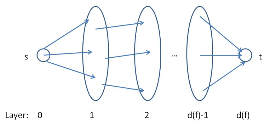
For the analysis, imagine running breadth-first search (BFS) in Gf starting from the
source s. Recall that BFS discovers vertices in “layers,” with s in the 0th layer, and layer
i + 1 consisting of those vertices not in a previous layer and reachable in one hop from a
vertex in the ith layer. We can then classify the edges of Gf as forward (meaning going from
layer i to layer i + 1, for some i), sideways (meaning both endpoints are in the same layer),
and backwards (traveling from a layer i to some layer j with j < i). By the definition of
breadth-first search, no forward edge of Gf can shortcut over a layer; every forward edge
goes only to the next layer.
We define L , with the L standing for “layered,” as the subgraph of G consisting only
f
of the forward edges (Figure 6). (Vertices in layers after the one containing t are irrelevant,
f
so they can be discarded if desired.)
Figure 6: Layered subgraph Lf
Why bother defining Lf ? Because it is a succinct encoding of all of the shortest s-t paths
of Gf — the paths on which the Edmonds-Karp algorithm might augment. Formally, every
s-t in Lf comprises only forward edges of the BFS and hence has exactly d(f) hops, the
minimum possible. Conversely, an s-t path that is in G but not L must contain at least
f
f
one detour (a sideways or backward edge) and hence requires at least d(f) + 1 hops to get
to t.
7
Any path with n or more edges has a repeated vertex, and deleted the corresponding cycle yields a path
with the same endpoints and fewer hops.
9

v
3
2
2
3
s
5
t
w
Figure 7: Example from first lecture. Initially, 0th layer is {s}, 1st layer is {v, w}, 2nd layer
is {t}.
v
1
2
3
2
s
5
t
2
w
Figure 8: Residual graph after sending flow on s → v → t. 0th layer is {s}, 1st layer is
{v, w}, 2nd layer is {t}.
v
1
2
2
s
5
t
1
2
2
w
Figure 9: Residual graph after sending additional flow on s → w → t. 0th layer is {s}, 1st
layer is {v}, 2nd layer is {w}, 3rd layer is {t}.
For example, let’s return to our first example in Lecture #1, shown in Figure 7. Let’s
watch how d(f) changes as we simulate the algorithm. Since we begin with the zero flow,
initially the residual graph Gf is the original graph G. The 0th layer is s, the first layer is
{
v, w}, and the second layer is t. Thus d(f) = 2 initially. There are two shortest paths,
1
0
s → v → t and s → w → t. Suppose the Edmonds-Karp algorithm chooses to augment on
the upper path, sending two units of flow. The new residual graph is shown in Figure 8. The
layers remain the same: {s}, {v, w}, and {t}, with d(f) still equal to 2. There is only one
shortest path, s → w → t. The Edmonds-Karp algorithm sends two units along this flow,
resulting in the new residual graph in Figure 9. Now, no two-hop paths remain: the first
layer contains only v, with w in second layer and t in the third layer. Thus, d(f) has jumped
from 2 to 3. The unique shortest path is s → v → w → t, and after the Edmonds-Karp
algorithm pushes one unit of flow on this path it terminates with a maximum flow.
Proof of Lemma 3.2: We start with part (a) of the lemma. Note that the only thing
we’re worried about is that an augmentation somehow introduces a new, shortest path that
shortcuts over some layers of Lf (as defined above).
Suppose the Edmonds-Karp algorithm augments the currents flow f by routing flow on
the path P. Because P is a shortest s-t path in G , it is also a path in the layered graph L .
f
f
The only new edges created by augmenting on P are edges that go in the reverse direction
of P. These are all backward edges, so any s-t of Gf that uses such an edge has at least
d(f) + 2 hops. Thus, no new shorter paths are formed in Gf after the augmentation.
Now consider a run of t iterations of the Edmonds-Karp algorithm in which the value of
d(f) = c stays constant. We need to show that t ≤ m. Before the first of these iterations,
we save a copy of the current layered network: let F denote the edges of L at this time,
f
and V = {s}, V , V , . . . , V the vertices if the various layers.8
0
1
2
c
Consider the first of these t iterations. As in the proof of part (a), the only new edges
introduced go from some Vi to Vi−1. By assumption, after the augmentation, there is still
an s-t path in the new residual graph with only c hops. Since no edge of of such a path can
shortcut over one of the layers V , V , . . . , V , it must consist only of edges in F. Inductively,
0
1
c
every one of these t iterations augments on a path consisting solely of edges in F. Each
such iteration zeroes out at least one edge e = (v, w) of F (the one with minimum residual
capacity), at which point edge e drops out of the current residual graph. The only way e
can reappear in the residual graph is if there is an augmentation in the reverse direction
(the direction (w, v)). But since (w, v) goes backward (from some Vi to Vi−1) and all of the
t iterations route flow only on edges of F (from some Vi to to Vi+1), this can never happen.
Since F contains at most m edges, there can only be m iterations before d(f) increases (or
the algorithm terminates). ꢀ
4
Dinic’s Algorithm: Blocking Flows
The next algorithm bears a strong resemblance to the Edmonds-Karp algorithm, though it
was developed independently and contemporaneously by Dinic. Unlike the Edmonds-Karp
algorithm, Dinic’s algorithm enjoys a modularity that lends itself to optimized algorithms
with faster running times.
8
The residual and layered networks change during these iterations, but F and V , . . . , V always refer to
0
c
networks before the first of these iterations.
1
1

Dinic’s Algorithm
initialize f = 0 for all e ∈ E
e
while there is an s-t path in the current residual network G do
f
construct the layered network L from G using breadth-first search,
f
f
as in the proof of Lemma 3.2
/ takes O(|E|) time
/
compute a blocking flow g (Definition 4.1) in Lf
/
/ augment the flow f using the flow g
for all edges (v, w) of G for which the corresponding forward edge
of Gf carries flow (gvw > 0) do
increase fe by ge
for all edges (v, w) of G for which the corresponding reverse edge
of Gf carries flow (gwv > 0) do
decrease fe by ge
Dinic’s algorithm can only terminate with a residual network with no s-t path, that is, with a
maximum flow (by Corollary 2.3). While in the Edmonds-Karp algorithm we only formed the
layered network Lf in the analysis (in the proof of Lemma 3.2), Dinic’s algorithm explicitly
constructs this network in each iteration.
A blocking flow is, intuitively, a bunch of shortest augmenting paths that get processed
as a batch. Somewhat more formally, blocking flows are precisely the possible outputs of the
naive greedy algorithm discussed at the beginning of Lecture #1. Completely formally:
Definition 4.1 (Blocking Flow) A blocking flow g in a network G is a feasible flow such
that, for every s-t path P of G, some edge e is saturated by g (i.e.,. f = u ).
e
e
That is, a blocking flow zeroes out an edge of every s-t path.
v
3
(3)
2
s
5 (3)
t
2
3 (3)
w
Figure 10: Example of blocking flow. This is not a maximum flow.
1
2


Recall from Lecture #1 that a blocking flow need not be a maximum flow; the blocking
flow in Figure 10 has value 3, while the maximum flow value is 5. While the blocking flow
in Figure 10 uses only one path, generally a blocking flow uses many paths. Indeed, every
flow that is maximum (equivalently, no s-t paths in the residual network) is also a blocking
flow (equivalently, no s-t paths in the residual network comprising only forward edges).
The running time analysis of Dinic’s algorithm is anchored by the following progress
lemma.
Lemma 4.2 (Dinic Progress Lemma) Fix a network G. For a flow f, let d(f) denote
the number of hops in a shortest s-t path (with positive residual capacity) in G , or +∞ if
f
no such paths exist (or +∞ if no such paths exist). If h is obtained from f be augmenting f
by a blocking flow g in G , then d(h) > d(f).
f
That is, every iteration of Dinic’s algorithm strictly increases the s-t distance in the current
residual graph.
We leave the proof of Lemma 4.2 as Exercise #5; the proof uses the same ideas as that
of Lemma 3.2. For an example, observe that after augmenting our running example by the
blocking flow in Figure 10, we obtain the residual network in Figure 11. We had d(f) = 2
initially, and d(f) = 3 after the augmentation.
v
3
2
2
3
s
2
3
t
w
Figure 11: Residual network of blocking flow in Figure 10. d(f) = 3 in this residual graph.
Since d(f) can only go up to n − 1 before becoming infinite (i.e., disconnecting s and t
in G ), Lemma 4.2 immediately implies that Dinic’s algorithm terminates after at most n
f
iterations. In this sense, the maximum flow problem reduces to n instances of the blocking
flow problem (in layered networks). The running time of Dinic’s algorithm is O(n · BF),
where BF denotes the running time required to compute a blocking flow in a layered network.
The Edmonds-Karp algorithm and its proof effectively shows how to compute a blocking
flow in O(m2) time, by repeatedly sending as much flow as possible on a single path of Lf
with positive residual capacity. On Problem Set #1 you’ll seen an algorithm, based on depth-
first search, that computes a blocking flow in time O(mn). With this subroutine, Dinic’s
1
3

algorithm runs in O(n2m) time, improving over the Edmonds-Karp algorithm. (Remember,
it’s always a win to replace an m with an n.)
Using fancy data structures, it’s known how to compute a maximum flow in near-linear
time (with just one extra logarithmic factor), yielding a maximum flow algorithm with run-
ning time close to O(mn). This running time is no longer so embarrassing, and resembles
time bounds that you saw in CS161, for example for the Bellman-Ford shortest-path algo-
rithm and for various all-pairs shortest paths algorithms.
5
Looking Ahead
Thus far, we focused on “augmenting path” maximum flow algorithms. Properly imple-
mented, such algorithms are reasonably practical. Our motivation here is pedagogical: these
algorithms remain the best way to develop your initial intuition about the maximum flow
problem.
Next lecture introduces a different paradigm for computing maximum flows, known as
the “push-relabel” framework. Such algorithms are reasonably simple, but somewhat less
intuitive than augmenting path algorithms. Properly implemented, they are blazingly fast
and are often the method of choice for solving the maximum flow problem in practice.
1
4
CS261: A Second Course in Algorithms
Lecture #3: The Push-Relabel Algorithm for Maximum
Flow∗
Tim Roughgarden†
January 12, 2016
1
Motivation
The maximum flow algorithms that we’ve studied so far are augmenting path algorithms,
meaning that they maintain a flow and augment it each iteration to increase its value. In
Lecture #1 we studied the Ford-Fulkerson algorithm, which augments along an arbitrary
s-t path of the residual networks, and only runs in pseudopolynomial time. In Lecture #2
we studied the Edmonds-Karp specialization of the Ford-Fulkerson algorithm, where in each
iteration a shortest s-t path in the residual network is chosen for augmentation. We proved
a running time bound of O(m2n) for this algorithm (as always, m = |E| and n = |V |).
Lecture #2 and Problem Set #1 discuss Dinic’s algorithm, where each iteration augments
the current flow by a blocking flow in a layered subgraph of the residual network. In Problem
Set #1 you will prove a running time bound of O(n2m) for this algorithm.
In the mid-1980s, a new approach to the maximum flow problem was developed. It is
known as the “push-relabel” paradigm. To this day, push-relabel algorithms are often the
method of choice in practice (even if they’ve never quite been the champion for the best
worst-case asymptotic running time).
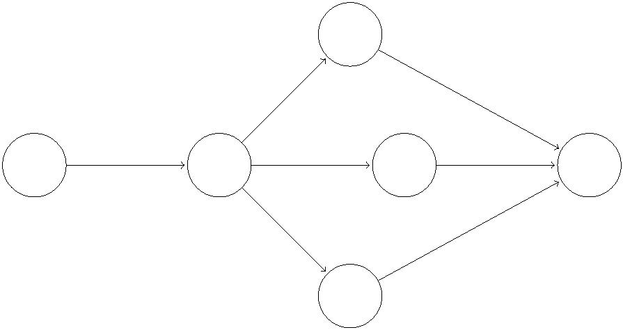
To motivate the push-relabel approach, consider the network in Figure 1, where k is a
large number (like 100,000). Observe the maximum flow value is k. The Ford-Fulkerson and
Edmonds-Karp algorithms run in Ω(k2) time in this network. Moreover, much of the work
feels wasted: each iteration, the long path of high-capacity edges has to be re-explored, even
though it hasn’t changed from the previous iteration. In this network, we’d rather route k
units of flow from s to x (in O(k) time), and then distribute this flow across the k paths from
∗
†
ꢀc
2
Department of Computer Science, Stanford University, 474 Gates Building, 353 Serra Mall, Stanford,
016, Tim Roughgarden.
CA 94305. Email: tim@cs.stanford.edu.
1

x to t (in O(k) time, linear-time overall). This is the idea behind push-relabel algorithms.1
Of course, if there were strictly less than k paths from x to t, then not all of the k units of
flow can be routed from x to t, and the remainder must be resent to the source. What is a
principled way to organize such a procedure in an arbitrary network?
v1
1
1
k
1
1
s
x
v2
t
1
1
vk
Figure 1: The edge {s, x} has a large capacity k, and there are k paths from x to t via
k different vertices v for 1 ≤ i ≤ k (3 are drawn for illustrative purposes). Both Ford-
i
Fulkerson and Edmonds-Karp take Ω(k2) time, but ideally we only need O(k) time if we can
somehow push k units of flow from s to x in one step.
2
Preliminaries
The first order of business is to relax the conservation constraints. For example, in Figure 1,
if we’ve routed k units of flow to x but not yet distributed over the paths to t, then the
vertex x has k units of flow incoming and zero units outgoing.
Definition 2.1 (Preflow) A preflow is a nonnegative vector {f }
that satisfies two con-
e
e∈E
straints:
Capacity constraints: f ≤ u for every edge e ∈ E;
e
e
Relaxed conservation constraints: for every vertex v other than s,
amount of flow entering v ≥ amount of flow exiting v.
The left-hand side is the sum of the fe’s over the edge incoming to v; likewise with the
outgoing edges for the right-hand side.
1
The push-relabel framework is not the unique way to address this issue. For example, fancy data
structures (“dynamic trees” and their ilk) can be used to remember the work performed by previous searches
and obtain faster running times.
2

The definition of a preflow is exactly the same as a flow (Lecture #1), except that the
conservation constraints have been relaxed so that the amount of flow into a vertex is allowed
to exceed the amount of flow out of the vertex.
We define the residual graph Gf with respect to a preflow f exactly as we did for the
case of a flow f. That is, for an edge e that carries flow f and capacity u , G includes a
e
e
f
forward version of e with residual capacity u − f and a reverse version of e with residual
e
capacity f . Edges with zero residual capacity are omitted from G .
e
e
f
Push-relabel algorithms work with preflows throughout their execution, but at the end
of the day they need to terminate with an actual flow. This motivates a measure of the
“
degree of violation” of the conservation constraints.
Definition 2.2 (Excess) For a flow f and a vertex v = s, t of a network, the excess αf (v)
is
amount of flow entering v − amount of flow exiting v.
For a preflow flow f, all excesses are nonnegative. A preflow is a flow if and only if the excess
of every vertex v = s, t is zero. Thus transforming a preflow to recover feasibility involves
reducing and eventually eliminating all excesses.
3
The Push Subroutine
How do we augment a preflow? When we were restricting attention to flows only, our hands
were tied — to maintain the conservation constraints, we only augmented along an s-t (or,
for a blocking flow, a collection of such paths). With the relaxed conservation constraints,
we have much more flexibility. All we need to is to augment a flow along a single edge at a
time, routing flow from one of its endpoints to the other.
Push(v)
choose an outgoing edge (v, w) of v in Gf (if any)
/
/ push as much flow as possible
let ∆ = min{α (v), resid. cap. of (v, w)}
f
push ∆ units of flow along (v, w)
The point of the second step is to send as much flow as possible from v to w using the edge
(v, w) of Gf , subject to the two constraints that define a preflow. There are two possible
bottlenecks. One is the residual capacity of the edge (v, w) (as dictated by nonnegativ-
ity/capacity constraints); if this binds, then the push is called saturating. The other is the
amount of excess at the vertex v (as dictated by the relaxed conservation constraints); if
this binds, the push is non-saturating. In the final step, the preflow is updated as in our
augmenting path algorithms: if (v, w) the forward version of edge e = (v, w) in G, then fe
is increased by ∆; if (v, w) the reverse version of edge e = (w, v) in G, then fe is decreased
by ∆. As always, the residual network is then updated accordingly. Note that after pushing
flow from v to w, w has positive excess (if it didn’t already).
3

4
Heights and Invariants
Just pushing flow around the residual network is not enough to obtain a correct maximum
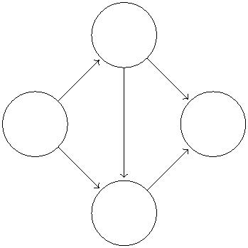
flow algorithm. One worry is illustrated by the graph in Figure 2 — after initially pushing
one unit flow from s to v, how do we avoid just pushing the excess around the cycle v →
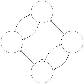
w → x → y → v forevermore. Obviously we want to push the excess to t when it gets to x,
but how can we be systematic about it?
v
y
s
t
w
x
Figure 2: When we push flows in the above graph, how do we ensure that we do not push
flows in the cycle v → w → x → y → v?
The next key idea will ensure termination of our algorithm, and will also implies correct-
ness as termination. The idea is to maintain a height h(v) for each vertex v of G. Heights
will always be nonnegative integers. You are encouraged to visualize a network in 3D, with
the height of a vertex giving it its z-coordinate, with edges going “uphill” and “downhill,”
or possibly staying flat. The plan for the algorithm is to always maintain three invariants
(two trivial and one non-trivial):
Invariants
1
2
3
. h(s) = n at all times (where n = |V |);
. h(t) = 0;
. for every edge (v, w) of the current residual network (with positive resid-
ual capacity), h(v) ≤ h(w) + 1.
Visually, the third invariant says that edges of the residual network are only to go downhill
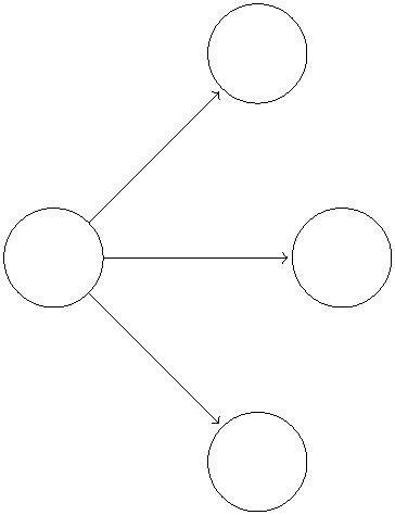
gradually (by one per hop). For example, if a vertex v has three outgoing edges (v, w1),
(v, w ), and (v, w ), with h(w ) = 3, h(w ) = 4, and h(w ) = 6, then the third invariant
2
3
1
2
3
requires that h(v) be 4 or less (Figure 3). Note that edges are allowed to go uphill, stay flat,
or go downhill (gradually).
4

w1
v
w2
w3
Figure 3: Given that h(w ) = 3, h(w ) = 4, h(w ) = 6, it must be that h(v) ≤ 4.
1
2
3
Where did these invariants come from? For one motivation, recall from Lecture #2 our
optimality conditions for the maximum flow problem: a flow is maximum if and only if there
is no s-t path (with positive residual capacity) in its residual graph. So clearly we want this
property at termination. The new idea is to satisfy the optimality conditions at all times,
and this is what the invariants guarantee. Indeed, since the invariants imply that s is at
height n, t is at height 0, and each edge of the residual graph only goes downhill by at
most 1, there can be no s-t path with at most n − 1 edges (and hence no s-t path at all).
It follows that if we find a preflow that is feasible (i.e., is actually a flow, with no excesses)
and the invariants hold (for suitable heights), then the flow must be a maximum flow.
It is illuminating to compare and contrast the high-level strategies of augmenting path
algorithms and of push-relabel algorithms.
Augmenting Path Strategy
Invariant: maintain a feasible flow.
Work toward: disconnecting s and t in the current residual network.
Push-Relabel Strategy
Invariant: maintain that s, t disconnected in the current residual network.
Work toward: feasibility (i.e., conservation constraints).
While there is a clear symmetry between the two approaches, most people find it less intuitive
to relax feasibility and only restore it at the end of the algorithm. This is probably why the
push-relabel framework only came along in the 1980s, while the augmenting path algorithms
we studied date from the 1950s-1970s. The idea of relaxing feasibility is useful for many
different problems.
5


In both cases, algorithm design is guided by an explicitly articulated strategy for guar-
anteeing correctness. The maximum flow problem, while polynomial-time solvable (as we
know), is complex enough that solutions require significant discipline. Contrast this with,
for example, the minimum spanning tree algorithms, where it’s easy to come up with cor-
rect algorithms (like Kruskal or Prim) without any advance understanding of why they are
correct.
5
The Algorithm
The high-level strategy of the algorithm is to maintain the three invariants above while trying
to zero out any remaining excesses. Let’s begin with the initialization. Since the invariants
reference both a correct preflow and current vertex heights, we need to initialize both. Let’s
start with the heights. Clearly we set h(s) = n and h(t) = 0. The first non-trivial decision
is to set h(v) = 0 also for all v = s, t. Moving onto the initial preflow, the obvious idea
is to start with the zero flow. But this violates the third invariant: edges going out of s
would travel from height n to 0, while edges of the residual graph are supposed to only go
downhill by 1. With the current choice of height function, no edges out of s can appear
(with non-zero capacity) in the residual network. So the obvious fix is to initially saturate
all such edges.
Initialization
set h(s) = n
set h(v) = 0 for all v = s
set f = u for all edges e outgoing from s
e
e
set fe = 0 for all other edges
All three invariants hold after the initialization (the only possible violation is the edges out
of s, which don’t appear in the initial residual network). Also, f is initialized to a preflow
(with flow in ≥ flow out except at s).
Next, we restrict the Push operation from Section 3 so that it maintains the invari-
ants. The restriction is that flow is only allowed to be pushed downhill in the residual
network.
Push(v) [revised]
choose an outgoing edge (v, w) of v in Gf with h(v) = h(w) + 1 (if any)
/
/ push as much flow as possible
let ∆ = min{α (v), resid. cap. of (v, w)}
f
push ∆ units of flow along (v, w)
Here’s the main loop of the push-relabel algorithm:
6


Main Loop
while there is a vertex v = s, t with αf (v) > 0 do
choose such a vertex v with the maximum height h(v)
/
/ break ties arbitrarily
if there is an outgoing edge (v, w) of v in Gf with h(v) = h(w) + 1
then
Push(v)
else
increment h(v)
// called a ‘‘relabel’’
Every iteration, among all vertices that have positive excess, the algorithm processes the
highest one. When such a vertex v is chosen, there may or may not be a downhill edge
emanating from v (see Figure 4(a) vs. Figure 4(b)). Push(v) is only invoked if there is
such an edge (in which case Push will push flow on it), otherwise the vertex is “relabeled,”
meaning its height is increased by one.
w1(3)
w1(3)
v(4)
w2(4)
v(2)
w2(4)
w3(6)
w3(6)
Figure 4: (a) v → w1 is downhill edge (4 to 3) (b) there are no downhill edges
Lemma 5.1 (Invariants Are Maintained) The three invariants are maintained through-
out the execution of the algorithm.
Neither s not t ever get relabeled, so the first two invariants are always satisfied. For
the third invariant, we consider separately a relabel (which changes the height function but
not the preflow) and a push (which changes the preflow but not the height function). The
only worry with a relabel at v is that, afterwards, some outgoing edge of v on the residual
network goes downhill by more than one step. But the precondition for relabeling is that all
outgoing edges are either flat or uphill, so this never happens. The only worry with a push
from v to w is that it could introduce a new edge (w, v) to the residual network that might
7


go downhill by more than one step. But we only push flow downward, so a newly created
reverse edge can only go upward.
The claim implies that if the push-relabel algorithm ever terminates, then it does so with
a maximum flow. The invariants imply the maximum flow optimality conditions (no s-t path
in the residual network), while the termination condition implies that the final preflow f is
in fact a feasible flow.
6
Example
Before proceeding to the running time analysis, let’s go through an example in detail to make
sure that the algorithm makes sense. The initial network is shown in Figure 5(a). After the
initialization (of both the height function and the preflow) we obtain the residual network
in Figure 5(b). (Edges are labeled with their residual capacities, vertices with both their
heights and their excesses.) 2
v(0, 1)
v
1
100
t(0)
1
100
1
100
s(4)
s
1
100
t
1
00
1
1
00
1
w(0, 100)
w
Figure 5: (a) Example network (b) Network after initialization. For v and w, the pair (a, b)
denotes that the vertex has height a and excess b. Note that we ignore excess of s and t, so
s and t both only have a single number denoting height.
In the first iteration of the main loop, there are two vertices with positive excess (v and
w), both with height 0, and the algorithm can choose arbitrarily which one to process. Let’s
process v. Since v currently has height 0, it certainly doesn’t have any outgoing edges in the
residual network that go down. So, we relabel v, and its height increases to 1. In the second
iteration of the algorithm, there is no choice about which vertex to process: v is now the
unique highest label with excess, so it is chosen again. Now v does have downhill outgoing
2
We looked at this network last lecture and determined that the maximum flow value is 3. So we should
be skeptical of the 100 units of flow currently on edge (s, w); it will have to return home to roost at some
point.
8

edges, namely (v, w) and (v, t). The algorithm is allowed to choose arbitrarily between such
edges. You’re probably rooting for the algorithm to push v’s excess straight to t, but to
keep things interesting let’s assume that that the algorithm pushes it to w instead. This is a
non-saturating push, and the excess at v drops to zero. The excess at w increases from 100
to 101. The new residual network is shown in Figure 6.
v(1, 0)
1
100
1
1
99
s(4)
t(0)
1
00
1
w(0, 101)
Figure 6: Residual network after non-saturating push from v to w.
In the next iteration, w is the only vertex with positive excess so it is chosen for processing.
It has no outgoing downhill edges, so it get relabeled (so now h(w) = 1). Now w does have a
downhill outgoing edge (w, t). The algorithm pushes one unit of flow on (w, t) — a saturating
push —- the excess at w goes back down to 100. Next iteration, w still has excess but has
no downhill edges in the new residual network, so it gets relabeled. With its new height
of 2, in the next iteration the edges from w to v go downhill. After pushing two units of flow
from w to v — one on the original (w, v) edge and one on the reverse edge corresponding
to (v, w) — the excess at w drops to 98, and v now again has an excess (of 2). The new
residual network is shown in Figure 7.
9
v(1, 2)
1
100
s(4)
1
100
t(0)
1
00
1
w(2, 98)
Figure 7: Residual network after non-saturating push from v to w.
Of the two vertices with excess, w is higher. It again has no downhill edges, however,
so the algorithm relabels it three times in a row until it does. When its height reaches 5,
the reverse edge (v, s) goes downhill, the algorithm pushes w’s entire excess to s. Now v is
the only vertex remaining with excess. Its edge (v, t) goes down hill, and after pushing two
units of flow on it the algorithm halts with a maximum flow (with value 3).
7
The Analysis
7
.1 Formal Statement and Discussion
Verifying that the push-relabel algorithm computes a maximum flow in one particular net-
work is all fine and good, but it’s not at all clear that it is correct (or even terminates) in
general. Happily, the following theorem holds.3
Theorem 7.1 The push-relabel algorithm terminates after O(n2) relabel operations and
O(n3) push operations.
The hidden constants in Theorem 7.1 are at most 2. Properly implemented, the push-relabel
algorithm has running time O(n3); we leave the details to Exercise Set #2. The one point
that requires some thought is to maintain suitable data structures so that a highest vertex
with excess can be identified in O(1) time.4 In practice, the algorithm tends to run in
sub-quadratic time.
A sharper analysis yields the better bound of O(n2√
m); see Problem Set #1. Believe it or now, the
3
√
worst-case running time of the algorithm is in fact Ω(n2 m).
Or rather, O(1) “amortized” time, meaning in total time O(n3) over all of the O(n3) iterations.
4
1
0


The proof of Theorem 7.1 is more indirect then our running time analyses of augmenting
path algorithms. In the latter algorithms, there are clear progress measures that we can use
(like the difference between the current and maximum flow values, or the distance between
s and t in the current residual network). For push-relabel, we require less intuitive progress
measures.
7
.2 Bounding the Relabels
The analysis begins with the following key lemma, proved at the end of the lecture.
Lemma 7.2 (Key Lemma) If the vertex v has positive excess in the preflow f, then there
is a path v s in the residual network Gf .
The intuition behind the lemma is that, since the excess for to v somehow from v, it should
be possible to “undo” this flow in the residual network.
For the rest of this section, we assume that Lemma 7.2 is true and use it to prove
Theorem 7.1. The lemma has some immediate corollaries.
Corollary 7.3 (Height Bound) In the push-relabel algorithm, every vertex always has
height at most 2n.
Proof: A vertex v is only relabeled when it has excess. Lemma 7.2 implies that, at this
point, there is a path from v to s in the current residual network Gf . There is therefore such
a path with at most n − 1 edges (more edges would create a cycle, which can be removed to
obtain a shorter path). By the first invariant (Section 4), the height of s is always n. By the
third invariant, edges of Gf can only go downhill by one step. So traversing the path from
v to s decreases the height by at most n − 1, and winds up at height n. Thus v has height
2
n − 1 or less, and at most one more than this after it is relabeled for the final time. ꢀ
The bound in Theorem 7.1 on the number of relabels follows immediately.
Corollary 7.4 (Relabel Bound) The push-relabel algorithm performs O(n2) relabels.
7
.3 Bounding the Saturating Pushes
We now bound the number of pushes. We piggyback on Corollary 7.4 by using the number
of relabels as a progress measure. We’ll show that lots of pushes happen only when there
are already lots of relabels, and then apply our upper bound on the number of relabels.
We handle the cases of saturating pushes (which saturate the edge) and non-saturating
pushes (which exhaust a vertex’s excess) separately.5 For saturating pushes, think about a
particular edge (v, w). What has to happen for this edge to suffer two saturating pushes in
the same direction?
5
To be concrete, in case of a tie let’s call it a non-saturating push.
1
1

Lemma 7.5 (Saturating Pushes) Between two saturating pushes on the same edge (v, w)
in the same direction, each of v, w is relabeled at least twice.
Since each vertex is relabeled O(n) times (Corollary 7.3), each edge (v, w) can only suffer
O(n) saturating pushes. This yields a bound of O(mn) on the number of saturating pushes.
Since m = O(n2), this is even better than the bound of O(n3) that we’re shooting for.6
Proof of Lemma 7.5: Suppose there is a saturating push on the edge (v, w). Since the push-
relabel algorithm only pushes downhill, v is higher than w (h(v) = h(w) + 1). Because the
push saturates (v, w), the edge drops out of the residual network. Clearly, a prerequisite
for another saturating push on (v, w) is for (v, w) to reappear in the residual network. The
only way this can happen is via a push in the opposite direction (on (w, v)). For this to
occur, w must first reach a height larger than that of v (i.e., h(w) > h(v)), which requires
w to be relabeled at least twice. After (v, w) has reappeared in the residual network (with
h(v) < h(w)), no flow will be pushed on it until v is again higher than w. This requires at
least two relabels to v. ꢀ
7
.4 Bounding the Non-Saturating Pushes
We now proceed to the non-saturating pushes. Note that nothing we’ve said so far relies
on our greedy criterion for the vertex to process in each iteration (the highest vertex with
excess). This feature of the algorithm plays an important role in this final step.
Lemma 7.6 (Non-Saturating Pushes) Between any two relabel operations, there are at
most n non-saturating pushes.
Corollary 7.4 and Lemma 7.6 immediately imply a bound of O(n3) on the number of non-
saturating pushes, which completes the proof of Theorem 7.1 (modulo the key lemma).
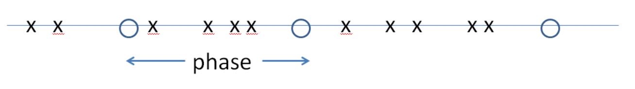
Proof of lemma 7.6: Think about the entire sequence of operations performed by the algo-
rithm. “Zoom in” to an interval bracketed by two relabel operations (possibly of different
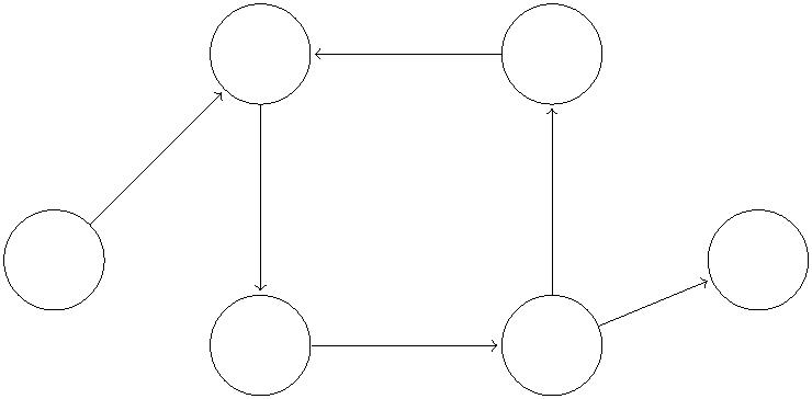
vertices), with no relabels in between. Call such an interval a phase of the algorithm. See
Figure 8.
6
We’re assuming that the input network has no parallel edges, between the same pair of vertices and in
the same direction. This is effectively without loss of generality — multiple edges in the same direction can
be replaced by a single one with capacity equal to the sum of the capacities of the parallel edges.
1
2

Figure 8: A timeline showing all operations (’O’ represents relabels, ’X’ represents non-
saturating pushes). An interval between two relabels (’O’s) is called a phase. There are
O(n2) phases, and each phase contains at most n non-saturating pushes.
How does a non-saturating push at a vertex v make progress? By zeroing out the excess
at v. Intuitively, we’d like to use the number of zero-excess vertices as a progress measure
within a phase. But a non-saturating push can create a new excess elsewhere. To argue that
this can’t go on for ever, we use that excess is only transferred from higher vertices to lower
vertices.
Formally, by the choice of v, as the highest vertex with excess, we have
h(v) ≥ h(w)
for all vertices w with excess
(1)
at the time of a non-saturating push at v. Inequality (1) continues to hold as long as there is
no relabel: pushes only send flow downhill, so can only transfer excess from higher vertices
to lower vertices.
After the non-saturating push at v, its excess is zero. How can it become positive again
in the future?7 It would have to receive flow from a higher vertex (with excess). This cannot
happen as long as (1) holds, and so can’t happen until there’s a relabel. We conclude that,
within a phase, there cannot be two non-saturating pushes at the same vertex v. The lemma
follows. ꢀ
7
.5 Analysis Recap
The proof of Theorem 7.1 has several cleverly arranged steps.
1
2
. Each vertex can only be relabeled O(n) times (Corollary 7.3 via Lemma 7.2),
for a total of O(n2) relabels.
. Each edge can only suffer O(n) saturating pushes (only 1 between each
time both endpoints are relabeled twice, by Lemma 7.5)), for a total of
O(mn) saturating pushes.
3
. Each vertex can only suffer O(n2) non-saturating pushes (only 1 per
phase, by Lemma 7.6), for a total of O(n3) such pushes.
7
For example, recall what happened to the vertex v in the example in Section 6.
1
3


8
Proof of Key Lemma
We now prove Lemma 7.2, that there is a path from every vertex with excess back to the
source s in the residual network. Recall the intuition: excess got to v from s somehow, and
the reverse edges should form a breadcrumb trail back to s.
Proof of Lemma 7.2: Fix a preflow f.8 Define
A = {v ∈ V : there is an s v path P in G with f > 0 for all e ∈ P}.
e
Conceptually, run your favorite graph search algorithm, starting from s, in the subgraph of
G consisting of the edges that carry positive flow. A is where you get stuck. (This is the
second example we’ve seen of the “reachable vertices” proof trick; there are many more.)
Why define A? Note that for a vertex v ∈ A, there is a path of reverse edges (with
positive residual capacity) from v to s in the residual network G . So we just have to prove
f
that all vertices with excess have to be in A.
Figure 9: Visualization of a cut. Recall that we can partition edges into 4 categories:(i)
edges with both endpoints in A; (ii) edges with both endpoints in B; (iii) edges sticking out
of B; (iv) edges sticking into B.
Define B = V − A. Certainly s is in A, and hence not in B. (As we’ll see, t isn’t in B
either.) We might have B = ∅ but this fine with us (we just want no vertices with excess in
B).
The key trick is to consider the quantity
X
[
flow out of v - flow in to v] .
(2)
|
The argument bears some resemblance to the final step of the proof of the max-flow/min-cut theorem
(Lecture #2) — the part where, given a residual network with no s-t path, we exhibited an s-t cut with
{z
}
v∈B
≤
0
8
value equal to that of the current flow.
1
4


Because f is a preflow (with flow in at least flow out except at s) and s ∈/ B, every term
of (2) is non-positive. On the other hand, recall from Lecture #2 that we can write the
sum in different way, focusing on edges rather than vertices. The partition of V into A and
B buckets edges into four categories (Figure 9): (i) edges with both endpoints in A; (ii)
edges with both endpoints in B; (iii) edges sticking out of B; (iv) edges sticking into B.
Edges of type (i) are clearly irrelevant for (2) (the sum only concerns vertices of B). An
edge e = (v, w) of type (ii) contributes the value fe once positively (as flow out of v) and once
negatively (as flow into w), and these cancel out. By the same reasoning, edges of type (iii)
and (iv) contribute once positively and once negatively, respectively. When the dust settles,
we find that the quantity in (2) can also be written as
X
X
f −
f ;
e
(3)
e
|
{z}
|{z}
e∈δ+(B)
e∈δ−(B)
≥
0
=0
recall the notation δ+(B) and δ (B) for the edges of G that stick out of and into B, respec-
−
tively. Clearly each term is the first sum is nonnegative. Each term is the second sum must
be zero: an edge e ∈ δ (B) sticks into A, so if f > 0 then the set A of vertices reachable by
−
e
flow-carrying edges would not have gotten stuck as soon as it did.
The quantities (2) and (3) are equal, yet one is non-positive and the other non-negative.
Thus, they must both be 0. Since every term in (2) is non-positive, every term is 0. This
implies that conservation constraints (flow in = flow out) hold for all vertices of B. Thus all
vertices with excess are in A. By the definition of A, there are paths of reverse edges in the
residual network from these vertices to s, as desired. ꢀ
1
5
CS261: A Second Course in Algorithms
Lecture #4: Applications of Maximum Flows and
Minimum Cuts∗
Tim Roughgarden†
January 14, 2016
1
From Algorithms to Applications
The first three lectures covered four maximum flow algorithms (Ford-Fulkerson, Edmonds-
Karp, Dinic’s blocking flow-based algorithm, and the Goldberg-Tarjan push-relabel algo-
rithm). We could talk about maximum flow algorithms til the cows come home — there
has been decades of intense work on the problem, including some interesting breakthroughs
just in the last couple of years. But four algorithms is enough for a course like CS261; it’s
time to move on to applications of the algorithms, and then on to study other fundamental
problems.
Let’s remind ourselves why we studied these algorithms.
1
. Often the best way to get a good understanding of a computational problem is to study
algorithms for it. For example, the Ford-Fulkerson algorithm introduced the crucial
concept of a residual network, and gave us an excellent initial feel for the maximum
flow problem.
2
3
. These algorithms are part of the canon, among the greatest hits of algorithms. So it’s
fun to know how they work.
. Maximum flow problems really do come up in practice, so it good to how you might
solve them quickly. The push-relabel algorithm is an excellent starting point for im-
plementing fast maximum flow algorithms.
The above reasons assume that we care about the maximum flow problem. And why do we
care? Because like all central algorithmic problems, it directly models several well-motivated
∗
†
ꢀc
2
Department of Computer Science, Stanford University, 474 Gates Building, 353 Serra Mall, Stanford,
016, Tim Roughgarden.
CA 94305. Email: tim@cs.stanford.edu.
1

problems (traffic in transportation networks, oil in a distribution network, data packets in a
communication network), and also a surprising number of problems are really just maximum
flow in disguise. The lecture gives two examples, in computer vision and in graph matching,
and the exercise and problem sets contain several more. Perhaps the most useful skill you
can learn in CS261, for both practical and theoretical work, is how to recognize when the
tools of the course apply. Hopefully, practice makes perfect.
2
The Minimum Cut Problem
Figure 1: Example of an (s, t)-cut.
The minimum (s, t)-cut problem made a brief cameo in Lecture #2. It is the “dual” problem
to maximum flow, in a sense we’ll make precise in later lectures, and it is just as ubiquitous
in applications. In the minimum (s, t)-cut problem, the input is the same as in the maximum
flow problem (a directed graph, source and sink vertices, and edge capacities). The feasible
solutions are the (s, t)-cuts, meaning the partitions of the vertex V into two sets A and B
with s ∈ A and t ∈ B (Figure 1). The objective is to compute the s-t cut with the minimum
capacity, meaning the total capacity on edges sticking out of the source-side of the cut (those
sticking in don’t count):
X
capacity of (A, B) =
u .
e
e∈δ+(a)
In Lecture #2 we noted a simple but extremely useful fact.
Corollary 2.1 The minimum s-t cut problem reduces in linear time to the maximum flow
problem.
Recall the argument: given a maximum flow, just do breadth- or depth-first search from s
in the residual graph (in linear time). We proved that if this search gets stuck at A, then
(A, V − A) is an (s, t)-cut with capacity equal to that of the flow; since no cut has capacity
less than any flow, the cut (A, V − A) must be a minimum cut.
2
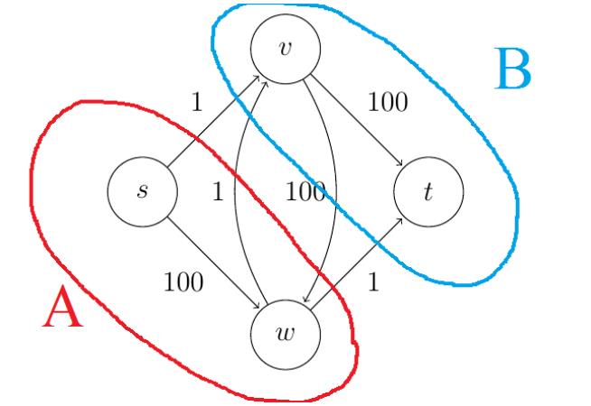
While there are some algorithms for solving the minimum (s, t)-cut problem without
going through maximum flows (especially for undirected graphs), in practice it is very com-
mon to solve it via this reduction. Next is an application of the problem to a basic image
segmentation task.
3
Image Segmentation
3
.1 The Problem
We consider the problem of classifying the pixels of an image as either foreground or back-
ground. We model the problem as follows. The input is an undirected graph G = (V, E),
where V is the set of pixels. The edges E designate pairs of pixels as neighbors. For example,
a common input is a grid graph (Figure 2(a)), with an edge between two pixels that different
by 1 in of the two coordinates. (Sometimes one also throws in the diagonals.) In any case,
the solution we present works no matter than the graph G is.
1
1
1
/0
/0
/0
1/0
0/1
1/0
1/0
1/0
1/0
Figure 2: Example of a grid network. In each vertex, first value denotes av and second value
denotes bv.
The input also contains 2|V | + |E| parameter values. Each vertex v is annotated with
two nonnegative numbers a and b , and each edge e has a nonnegative value p . We discuss
v
the semantics of these shortly.
v
e
The feasible outputs are the partitions V into a foreground X and background Y ; it’s
OK if X or Y is empty. We assess the quality of a solution by the objective function
X
X
X
av +
bv −
p ,
e
(1)
v∈X
v∈Y
e∈δ(X)
which we want to make as large as possible. (δ(X) denotes the edges cut by the partition
(X, Y ), with one endpoint on each side.)
3
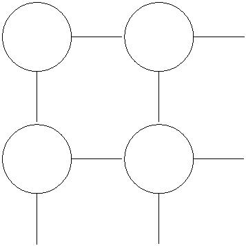
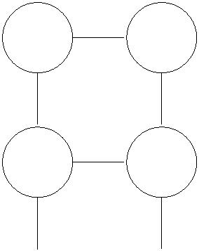
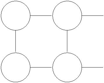
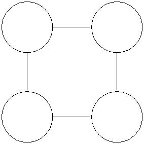
We see that a vertex v earns a “prize” of a if it is included in X and b otherwise. In
v
v
practice, these parameter values come from a prior as to whether a pixel v is more “likely” to
be in the foreground (in which case a is big and b small) or in the background (leading to
v
a big b and small a . It’s not important for our purposes how this prior or these parameter
v
v
v
are chosen, but it’s easy to imagine examples. Perhaps a light blue pixel is typically part
of the background (namely, the sky). Or perhaps one already knows a similar image that
has already been segmented, like one taken earlier from the same position, and then declares
that each pixel’s region is likely to be the same as in the reference image.
If all we had were the a’s and b’s, the problem would be trivial — independently for
each pixel, you would just assign it optimally to either X (if a > b ) or Y (if b > a ).
v
v
v
v
The point of the neighboring relation E is that we also expect that images are mostly
“
smooth,” with neighboring pixels much more likely to be in the same region than in different
regions. The penalty pe is incurred whenever the endpoints of e violate this prior belief. In
machine learning terminology, the final objective (1) corresponds to a massaged version of
the “maximum likelihood” objective function.
For example, suppose all pe’s are 0 in Figure 2(a). Then, the optimal solution assigns the
entire boundary to the foreground and the middle pixel to the background. The objective
function would be 9. If all the pe’s were 1, however, then this feasible solution would have
value only 5 (because of the four cut edges). The optimal solution assigns all 9 pixels to the
foreground, for a value of 8. The latter computation effectively recovers a corrupted pixel
inside some homogeneous region.
3
.2 Toward a Reduction
Theorem 3.1 The image segmentation problem reduces, in linear time, to the minimum
(s, t)-cut problem (and hence to the maximum flow problem).
How would one ever suspect that such a reduction exists? The big clue is the form of the
output of the image segmentation problem, as the partition of a vertex set into two pieces.
This sure sounds like a cut problem. The coolest thing that could be true is that the problem
reduces to a cut problem that we already know how to solve, like the minimum (s, t)-cut
problem.
Digging deeper, there are several differences between image segmentation and (s, t)-cut
that might give us pause (Table 1). For example, while both problems have one parameter
per edge, the image segmentation problem has two parameters per vertex that seem to have
no analog in the minimum (s, t)-cut problem. Happily, all of these issues can be addressed
with the right reduction.
4
Minimum (s, t)-cut Image segmentation
minimization objective maximization objective
source s, sink t
directed
no vertex parameters
no source, sink vertices
undirected
a , b for each v ∈ V
v
v
Table 1: Differences between the image segmentation problem and the minimum (s, t)-cut
problem.
3
.3 Transforming the Objective Function
First, it’s easy to convert the maximization objective function into a minimization one by
multiplying through by -1:
X
X
X
min
(X,Y )
pe −
av −
b .
v
e∈δ(X)
v∈X
vinY
Clearly, the optimal solution under this objective is the same as under the original objective.
It’s hard not to be a little spooked by the negative numbers in this objective function
(e.g., in max flow or min cut, edge capacities are always nonnegative). This is also easy to
P
P
fix. We just shift the objective function by adding the constant value
every feasible solution. This gives the objective function
av +
bv to
v∈V
v
∈
V
X
X
X
min
(X,Y )
pe +
av +
b .
v
(2)
e∈δ(X)
v∈Y
vinX
Since we shifted all feasible solutions by the same amount, the optimal solution remains
unchanged.
3
.4 Transforming the Graph
We use tricks familiar from Exercise Set #1. Given the undirected graph G = (V, E), we
0
construct a directed graph G = (V , E ) as follows:
0
0
•
•
V 0 = V ∪ {s, t} (i.e., add a new source and sink)
E0 has two bidirected edges for each edge e in E (i.e., a directed edge in either direction).
The capacity of both directed edges is defined to be pe, the given penalty of edge e
(Figure 3).
5

pe
pe
v
w
pe
v
w
Figure 3: The (undirected) edges of G are bidirected in G0.
•
E0 also has an edge (s, v) for every pixel v ∈ V , with capacity u = a .
sv
v
•
E0 has an edge (v, t) for every pixel v ∈ V , with capacity u = b .
See Figure 4 for a small example of the transformation.
vt
v
a
c
s
t
a
b
c
b
d
d
Figure 4: (a) initial network and (b) the transformation
3
.5 Proof of Theorem 3.1
Consider an input G = (V, E) to the image segmentation problem and directed graph G0 =
0
0
(V , E ) constructed by the reduction above. There is a natural bijection between partitions
t . The key claim
∪ { }
(X, Y ) of V and (s, t)-cut (A, B) of G0, with A
↔
X
s and B
∪ { }
↔
Y
is that this correspondence preserves objective function value — that the capacity of every
(s, t)-cut (A, B) of G0 is precisely the objective function value (under (2))of the partition
(A \ {s}, B \ {t}).
So fix an (s, t)-cut (X ∪ {s}, Y ∪ {t}) of G0. Here are the edges sticking out of X
s :
∪ { }
1
. for every v ∈ Y , δ+(X ∪ {s}) contains the edge (s, v), which has capacity av;
6

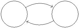
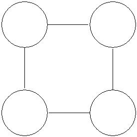
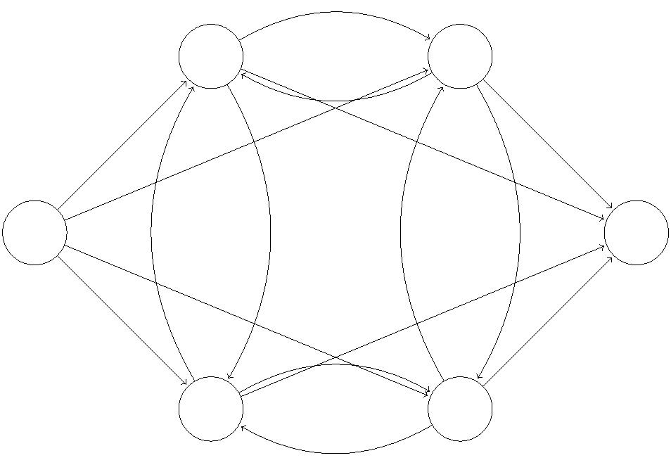
2
3
. for every v ∈ X, δ+(X ∪ {s}) contains the edge (v, t), which has capacity bv;
. for every edge e ∈ δ(X), δ+(X ∪ {s}) contains exactly one of the two corresponding
0
directed edges of G (the other one goes backward), and it has capacity p .
e
These are precisely the edges of δ+(X∪{s}). We compute the cut’s capacity just be summing
up, for a total of
X
X
X
av +
bv +
p .
e
v∈Y
v∈X
e∈δ(X)
This is identical to the objective function value (2) of the partition (X, Y ). We conclude
that computing the optimal such partition reduces to computing a minimum (s, t)-cut of G0.
The reduction can be implemented in linear time.
4
Bipartite Matching
Figure 5: Visualization of bipartite graph. Edges exist only between the partitions V and
W.
We next give a famous application of maximum flow. This application also serves as a segue
between the first two major topics of the course, the maximum flow problem and graph
matching problems.
In the bipartite matching problem, the input is an undirected bipartite graph G = (V ∪
W, E), with every edge of E having one endpoint in each of V and W. That is, no edges
internal to V or W are allowed (Figure 5). The feasible solutions are the matchings of the
graph, meaning subsets S ⊆ E of edges that share no endpoints. The goal of the problem is
to compute a matching with the maximum-possible cardinality. Said differently, the goal is
to pair up as many vertices as possible (using edges of E).
For example, the square graph (Figure 6(a)) is bipartite, and the maximum-cardinality
matching has size 2. It matches all of the vertices, which is obviously the best-case scenario.
Such a matching is called perfect.
7
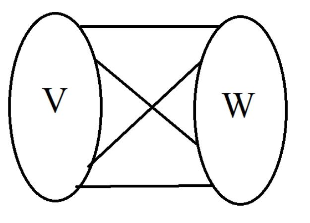
a
b
c
a
b
c
a
b
c
d
d
Figure 6: (a) square graph with perfect matching of 2. (b) star graph with maximum-
cardinality matching of 1. (c) non-bipartite graph with maximum matching of 1.
Not all graphs have perfect matchings. For example, in the star graph (Figure 6(b)),
which is also bipartite, no many how many vertices there are, the maximum-cardinality
matching has size only 1.
It’s also interesting to discuss the maximum-cardinality matching problem in general
(non-bipartite) graphs (like Figure 6(c)), but this is a harder topic that we won’t cover here.
While one can of course consider the bipartite special case of any graph problem, in matching
bipartite graphs play a particularly fundamental role. First, matching theory is nicer and
matching algorithms are faster for bipartite graphs than for non-bipartite graphs. Second, a
majority of the applications of already in the bipartite special case — assigning workers to
jobs, courses to room/time slots, medical residents to hospitals, etc.
Claim: maximum-cardinality matching reduces in linear time to maximum flow.
Proof sketch: Given an undirected bipartite graph (V ∪W, E), construct a directed graph
0
0
∪
∪{
}
G as in Figure 7(b). We add a source and sink, so the new vertex set is V = V
W
s, t .
0
To obtain E from E, we direct all edges of G from V to W and also add edges from s to
every vertex of V and from every vertex of W to t. Edges incident to s or t have capacity 1,
reflecting the constraints the each vertex of V ∪ W can only be matches to one other vertex.
Each edge (v, w) directed from V to W can be given any capacity that is at least 1 (v can
only receive one unit of flow, anyway); for simplicity, give all these edges infinite capacity.
You should check that there is a one-to-one correspondence between matchings of G and
integer-valued flows in G0, with edge (v, w) corresponding to one unit of flow on the path
s → v → w → t in G (Figure 7). This bijection preserves the objective function value.
0
0
Thus, given an integral maximum flow in G , the edges from V to W that carry flow form a
maximum matching.1
1
All of the maximum flow algorithms that we’ve discussed return an integral maximum flow provided all
the edge capacities are integers. The reason is that inductively, the current (pre)flow, and hence the residual
capacities, and hence the augmentation amount, stay integral throughout these algorithms.
8

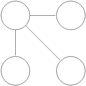
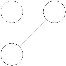

∞
u
v
w
x
1
1
u
v
w
x
∞
∞
s
t
1
1
Figure 7: (a) original bipartite graph G and (b) the constructed directed graph G. There is
one-to-one correspondence between matchings of G and integer-valued flows of G0 e.g. (v, w)
in G corresponds to one unit of flow on s → v → w → t in G0.
5
Hall’s Theorem
In this final section we tie together a number of courses ongoing themes. We previously
asked the question
How do we know when we’re done (i.e., optimal)?
for the maximum flow problem. Let’s ask it again for the maximum-cardinality bipartite
matching problem. Using the reduction in Section 4, we can translate the optimality con-
ditions for the maximum flow problem (i.e., the max-flow/min-cut theorem) into a famous
optimality condition for bipartite matchings.
Consider a bipartite graph G = (V ∪ W, E) with |V | ≤ |W|, renaming V, W if necessary.
Call a matching of G perfect if it matches every vertex in V ; clearly, a perfect matching is a
maximum matching. Let’s first understand which bipartite graphs admit a perfect matching.
Some notation: for a subset S ⊆ V , let N(S) denote the union of the neighborhoods of
the vertices of S: N(S) = {w ∈ W : ∃v ∈ S s.t. (v, w) ∈ E}. See Figure 8 for two examples
of such neighbor sets.
9
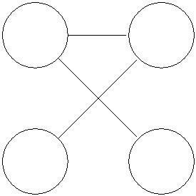
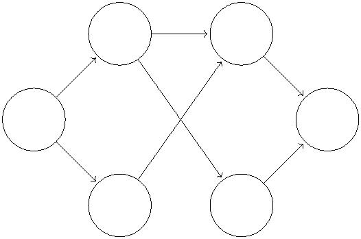
S
S
S
T
T
N(S)
N(S)
N(T)
N(T)
N(T)
N(T)
Figure 8: Two examples of vertex sets S and T and their respective neighbour sets N(S)
and N(T).
Does the graph in Figure 8 have a perfect matching? A little thought shows that the
answer is “no.” The three vertices of S have only two distinct neighbors between them.
Since each vertex can only be matched to one other vertex, there is no hope of matching
more than two of the three vertices of S.
More generally, if a bipartite graph has a constricting set S ⊆ V , meaning one with
|
N(S)| < |S|, then it has no perfect matching. But what about the converse? If a bipartite
graph admits no perfect matching, can you always find a short convincing argument of this
fact, in the form of a constricting set? Or could there be obstructions to perfect matchings
beyond just constricting sets? Hall’s Theorem gives the beautiful answer that constricting
sets are the only obstacles to perfect matchings.2
Theorem 5.1 (Hall’s Theorem) A bipartite graph (V ∪ W, E) with |V | ≤ |W| has a per-
fect matching if and only if, for every subset S ⊆ V , |N(S)| ≥ |S|.
2
Hall’s theorem actually predates the max-flow/min-cut theorem by 20 years.
1
0
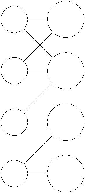
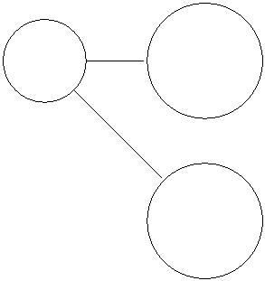

Thus, it’s not only easy to convince someone that a graph has a perfect matching (just
exhibit a matching), it’s also easy to convince someone that a graph does not have a perfect
matching (just exhibit a constricting set).
Proof of Theorem 5.1: We already argued the easy “only if” direction. For the “if” direction,
suppose that |N(S)| ≥ |S| for every S ⊆ V .
Claim: in the flow network G0 that corresponds to G (Figure 7), every (s, t)-cut has
capacity at least |V |.
To see why the claim implies the theorem, note that it implies that the minimum cut
0
value in G is at least V , so the maximum flow in G is at least V (by the max-flow/min-cut
| |
0
| |
theorem), and an integral flow with value |V | corresponds to a perfect matching of G.
Proof of claim: Fix an (s, t)-cut (A, B) of G0. Let S = A V denote the vertices of
V that lie on the source side. Since s ∈ A, all (unit-capacity) edges from s to vertices of
V − A contribute to the capacity of (A, B). Recall that we gave the edges directed from V
to W infinite capacity. Thus, if some vertex w of N(S) fails to also be in A, then the cut
(A, B) has infinite capacity (because of the edge from S to w) and there is nothing to prove.
So suppose all of N(S) belongs to A. Then all of the (unit-capacity) edges from vertices of
N(S) to t contribute to the capacity of (A, B). Summing up, we have
∩
capacity of (A, B) ≥ (|V | − |S|)
+
|N(S)|
edges from N(S) to t
|
{z
}
| {z }
edges from s to V − S
≥
|V |,
(3)
where (3) follows from the assumption that |N(S)| ≥ |S| for every S ⊆ V . ꢀ
On Exercise Set #2 you will extend this proof to show that, more generally, for every
bipartite graph (V ∪ W, E) with |V | ≤ |W|,
size of maximum matching = mS⊆iVn (|V | − (|S| − |N(S)|)) .
Note that at least |S| − |N(S)| vertices of S are unmatched in every matching.
1
1


CS261: A Second Course in Algorithms
Lecture #5: Minimum-Cost Bipartite Matching∗
Tim Roughgarden†
January 19, 2016
1
Preliminaries
a
b
c
d
Figure 1: Example of bipartite graph. The edges {a, b} and {c, d} constitute a matching.
Last lecture introduced the maximum-cardinality bipartite matching problem. Recall that
a bipartite graph G = (V ∪ W, E) is one whose vertices are split into two sets such that
every edge has one endpoint in each set (no edges internal to V or W allowed). Recall that
a matching is a subset M ⊆ E of edges with no shared endpoints (e.g., Figure 1). Last
lecture, we sketched a simple reduction from this problem to the maximum flow problem.
Moreover, we deduced from this reduction and the max-flow/min-cut theorem a famous
optimality condition for bipartite matchings. A special case is Hall’s theorem, which states
that a bipartite graph with |V | ≤ |W| has a perfect matching if and only if for every subset
S ⊆ V of the left-hand side, the number |N(S)| of S on the right-hand side is at least |S|.
See Problem Set #2 for quite good running time bounds for the problem.
But what if a bipartite graph has many perfect matchings? In applications, there are
often reasons to prefer one over another. For example, when assigning jobs to works, perhaps
there are many workers who can perform a particular job, but some of them are better at
∗
†
ꢀc
2
Department of Computer Science, Stanford University, 474 Gates Building, 353 Serra Mall, Stanford,
016, Tim Roughgarden.
CA 94305. Email: tim@cs.stanford.edu.
1


it than others. The simplest way to model such preferences is attach a cost ce to each edge
e ∈ E of the input bipartite graph G = (V ∪ W, E).
We also make three assumptions. These are for convenience, and are not crucial for any
of our results.
1
. The sets V and W have the same size, call it n. This assumption is easily enforced by
adding “dummy vertices” (with no incident edges) to the smaller side.
2
. The graph G has at least one perfect matching. This is easily enforced by adding
“dummy edges” that have a very high cost (e.g., one such edge from the ith vertex of
V to the ith vertex of W, for each i).
3
. Edge costs are nonnegative. This can be enforced in the obvious way: if the most
negative edge cost is −M, just add M to the cost of every edge. This adds the same
number (nM) to every perfect matching, and thus does not change the problem.
The goal in the minimum-cost perfect bipartite matching problem is to compute the perfect
matching M that minimizes
P
ce. The feasible solutions to the problem are the perfect
e∈M
matchings of G. An equivalent problem is the maximum-weight perfect bipartite matching
problem (just multiply all weights by −1 to transform them into costs).
When every edge has the same cost and we only care about cardinality, the problem
reduces to the maximum flow problem (Lecture #4). With general costs, there does not
seem to be a natural reduction to the maximum flow problem. It’s true that edges in a flow
network come with attached numbers (their capacities), but there is a type mismatch: edge
capacities affect the set of feasible solutions but not their objective function values, while
edge costs do the opposite. Thus, the minimum-cost perfect bipartite matching problem
seems like a new problem, for which we have to design an algorithm from scratch.
We’ll follow the same kind of disciplined approach that served us so well in the maximum
flow problem. First, we identify optimality conditions, which tell us when a given perfect
matching is in fact minimum-cost. This step is structural, not algorithmic, and is analogous
to our result in Lecture #2 that a flow is maximum if and only if there is no s-t path in the
residual network. Then, we design an algorithm that can only terminate with the feasibility
and optimality conditions satisfied. For maximum flow, we had one algorithmic paradigm
that maintained feasibility and worked toward the optimality conditions (augmenting path
algorithms), and a second paradigm that maintain the optimality conditions and worked
toward feasibility (push-relabel). Here, we follow the second approach. We’ll identify invari-
ants that imply the optimality condition, and design an algorithm that keeps them satisfied
at all times and works toward a feasible solution (i.e., a perfect matching).
2
Optimality Conditions
How do we know if a given perfect matching has the minimum-possible cost? Optimality
conditions are different for different problems, but for the problems studied in CS261 they are
2
all quite natural in hindsight. We first need an analog of a residual network. This requires
some definitions (see also Figure 2).
7
a
b
c
5
6
d
2
Figure 2: If our matching contains {a, b} and {c, d}, then a → b → d → c → a is both an
M-alternating cycle and a negative cycle.
Definition 2.1 (Negative Cycle) Let M be a matching in the bipartite graph G = (V ∪
W, E).
(a) A cycle C of G is M-alternating if every other edge of C belongs to M (Figure 2).1
(b) An M-alternating cycle is negative if the edges in the matching have higher cost than
those outside the matching:
X
X
ce >
c .
e
e∪C∩M
e∈C\M
Otherwise, it is nonnegative.
One interesting thing about alternating cycles is that by “toggling” the edges of C with
respect to M — that is, removing the edges of C ∩M and plugging in the edges of C \M —
0
yields a new matching M that matches exactly the same set of vertices. (Vertices outside
of C are clearly unaffected; vertices inside C remain matched to precisely one other vertex
of C, just a different one than before.)
Suppose M is a perfect matching, and we toggle the edges of an M-alternating cycle
0
to get another (perfect) matching M . Dropping the edges from C M saves us a cost of
∩
P
P
c , while adding the edges of C \ M cost us
c . Then M has smaller cost
C M
0
e∪C∩M
e
than M if and only if C is a negative cycle.
e
∈
\
e
The point of a negative cycle is that it offers a quick and convincing proof that a per-
fect matching is not minimum-cost (since toggling the edges of the cycle yields a cheaper
matching). But what about the converse? If a perfect matching is not minimum-cost, are
we guaranteed such a short and convincing proof of this fact? Or are there “obstacles” to
optimality beyond the obvious ones of negative cycles?
1
Since G is bipartite, C is necessarily an even cycle. One certainly can’t have more than every other edge
of C contained in the matching M.
3


Theorem 2.2 (Optimality Conditions for Min-Cost Bipartite Matching) A perfect
matching of a bipartite graph has minimum-cost if and only if there is no negative M-
alternating cycle.
Proof: We have already argued the “only if” direction. For the harder “if” direction, suppose
0
that M is a perfect matching and that there is no negative M-alternating cycle. Let M
be any other perfect matching; we want to show that the cost of M0 is at least that of M.
Consider M ⊕ M , meaning the symmetric difference of M, M (if you want to think of them
0
0
as sets) or their XOR (if you want to think of them as 0/1 vectors). See Figure 3 for two
examples.
a
c
e
a
c
e
a
c
e
b
d
c
f
e
b
d
c
f
e
b
d
c
f
e
⊕
⊕
=
=
a
a
a
b
d
f
b
d
f
b
d
f
Figure 3: Two examples that show what happens when we XOR two matchings (the dashed
edges).
In general, M ⊕ M is a union of (vertex-)disjoint cycles. The reason is that, since every
0
0
vertex has degree 1 in both M and M , every vertex of v has degree either 0 (if it is matched
to the same vertex in both M and M0) or 2 (otherwise). A graph with all degrees either 0
or 2 must be the union of disjoint cycles.
Since taking the symmetric difference/XOR with the same set two times in a row recovers
0
the initial set, (M ⊕ M ) M0 = M. Since M M0 is a disjoint union of cycles, taking the
⊕
⊕
symmetric different/XOR with M ⊕ M just means toggling the edges in each of its cycles
(since they are disjoint, they don’t interfere and the toggling can be done in parallel). Each
of these cycles is M-alternating, and by assumption each is nonnegative. Thus toggling the
0
0
0
edges of the cycles can only produce a more expensive perfect matching M . Since M was
an arbitrary perfect matching, M must be a minimum-cost perfect matching. ꢀ
4
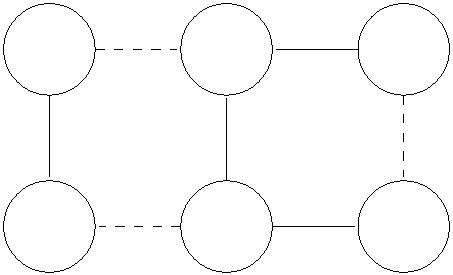
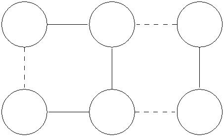
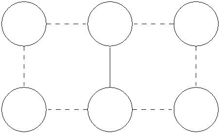

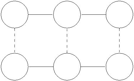
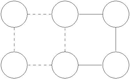
3
Reduced Costs and Invariants
Now that we know when we’re done, we work toward algorithms that terminate with the
optimality conditions satisfied. Following the push-relabel approach (Lecture #3), we next
identify invariants that will imply the optimality conditions at all times. Our algorithm will
maintain these as it works toward a feasible solution (i.e., a perfect matching). Continuing
the analogy with the push-relabel paradigm, we maintain a extra number pv for each vertex
v ∈ V ∪ W, called a price (analogous to the “heights” in Lecture #3). Prices are allowed to
be positive or negative. We use prices to force us to add edges to our current matching only
in a disciplined way, somewhat analogous to how we only pushed flow “downhill” in Lecture
#
3.
Formally, for a price vector p (indexed by vertices), we define the reduced cost of an edge
e = (v, w) by
p
e
c = c − p − p .
Here are our invariants, which are respect to a current matching M and a current vector p
(1)
e
v
w
of prices.
Invariants
1
2
. Every edge of G has nonnegative reduced cost.
. Every edge of M is tight, meaning it has zero reduced cost.
7
7
v(7)
w(0)
v(5)
w(2)
y(0)
5
5
6
6
x(2)
y(0)
x(2)
2
2
Figure 4: For the given (perfect) matching (dashed edges), (a) violates invariant 1, while (b)
satisfies all invariants.
For example, consider the (perfect) matching in Figure 4. Is it possible to define prices
so that the invariants hold? To satisfy the second invariant, we need to make the edges
(v, w) and (x, y) tight. We could try setting the price of w and y to 0, which then dictates
setting p = 7 and p = 2 (Figure 4(a)). This violates the first invariant, however, since
v
x
the reduced cost of edge (v, y) is -1. We can satisfy both invariants by resetting pv = 5 and
pw = 2; then both edges in the matching are tight and the other two edges have reduced
cost 1 (Figure 4(b)).
5


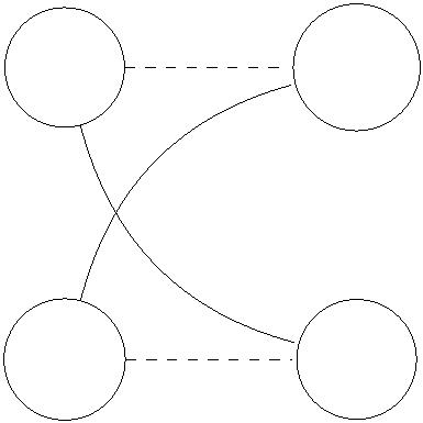
The matching in Figure 4 is a min-cost perfect matching. This is no coincidence.
Lemma 3.1 (Invariants Imply Optimality Condition) If M is a perfect matching and
both invariants hold, then M is a minimum-cost perfect matching.
Proof: Let M be a perfect matching such that both invariants hold. By our optimality
condition (Theorem 2.2), we just need to check that there is no negative cycle. So consider
any M-alternating cycle C (remember a negative cycle must be M-alternating, by definition).
We want to show that the edges of C that are in M have cost at most that of the edges of
P
C not in M. Adding and subtracting
pv and using the fact that every vertex of C is
v∈C
the endpoint of exactly one edge of C ∩ M and of C \ M (e.g., Figure 5), we can write
X
X
X
X
p
e
ce =
c +
pv
(2)
(3)
e∈C∩M
e∈C∩M
v∈C
and
X
X
p
e
ce =
c +
p .
v
e∈C\M
e∈C\M
v∈C
(We are abusing notation and using C both to denote the vertices in the cycle and the edges
in the cycle; hopefully the meaning is always clear from context.) Clearly, the third terms
in (2) and (3) are the same. By the second invariant (edges of M are tight), the second term
in (2) is 0. By the first invariant (all edges have nonnegative reduced cost), the second term
in (3) is at least 0. We conclude that the left-hand side of (2) is at most that of (3), which
proves that C is not a negative cycle. Since C was arbitrary M-alternating cycle, the proof
is complete. ꢀ
b
d
a
f
c
e
Figure 5: In the example M-alternating cycle and matching shown above, every vertex is an
endpoint of exactly one edge in M and one edge not in M.
4
The Hungarian Algorithm
Lemma 3.1 reduces the problem of designing a correct algorithm for the minimum-cost
perfect bipartite matching problem to that of designing an algorithm that maintains the
two invariants and computes an arbitrary perfect matching. This section presents such an
algorithm.
6
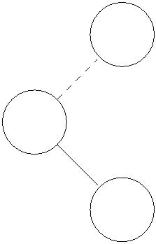
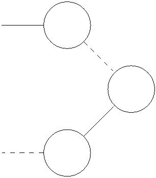
4
.1 Backstory
The algorithm we present goes by various names, the two most common being the Hungarian
algorithm and the Kuhn-Munkres algorithm. You might therefore find it weird that Kuhn
and Munkres are American. Here’s the story. In the early/mid-1950s, Kuhn really wanted
an algorithm for solving the minimum-cost bipartite matching problem. So he was reading
a graph theory book by K˝onig. This was actually the first graph theory book ever written
—
in the 1930s, and available in the U.S. only in 1950 (even then, only in German). Kuhn
was intrigued by an offhand citation in the book, to a paper of Egerv´ary. Kuhn tracked
down the paper, which was written in Hungarian. This was way before Google Translate, so
he bought a big English-Hungarian dictionary and translated the whole thing. And indeed,
Egerva´ry’s paper had the key ideas necessary for a good algorithm. K˝onig and Egerva´ry were
both Hungarian, so Kuhn called his algorithm the Hungarian algorithm. Kuhn only proved
termination of his algorithm, and soon thereafter Munkres observed a polynomial time bound
(basically the bound proved in this lecture). Hence, also called the Kuhn-Munkres algorithm.
In a (final?) twist to the story, in 2006 it was discovered that Jacobi, the famous math-
ematician (you’ve studied multiple concepts named after him in your math classes), came
up with an equivalent algorithm in the 1840s! (Published only posthumously, in 1890.)
Kuhn, then in his 80s, was a good sport about it, giving talks with the title “The Hungarian
Algorithm and How Jacobi Beat Me By 100 Years.”
4
.2 The Algorithm: High-Level Structure
The Hungarian algorithm maintains both a matching M and prices p. The initialization is
straightforward.
Initialization
set M = ∅
set p = 0 for all v ∈ V ∪ W
v
The second invariant holds vacuously. The first invariant holds because we are assuming
that all edge costs (and hence initial reduced costs) are nonnegative.
Informally (and way underspecified), the main loop works as follows. The terms “aug-
ment,” “good path,” and “good set” will be defined shortly.
Main Loop (High-Level)
while M is not a perfect matching do
if there is a good path P then
augment M by P
else
find a good set S; update prices accordingly
7


4
.3 Good Paths
We now start filling in the details. Fix the current matching M and current prices p. Call a
path P from v to w good if:
1
2
3
. both endpoints v, w are unmatched in M, with v ∈ V and w ∈ W (hence P has odd
length);
. it alternates edges out of M with edges in M (since v, w are unmatched, the first and
last edges are not in M);
. every edge of P is tight (i.e., has zero reduced cost and hence eligible to be included
in the current matching).
Figure 6 depicts a simple example of a good path.
4
a(2)
b(2)
c(2)
d(2)
4
4
4
Figure 6: Dashed edges denote edges in the matching and red edges denote a good path.
The reason we care about good paths is that such a path allows us to increase the
cardinality of M without breaking either invariant. Specifically, consider replacing M by
M0 = M P. This can be thought of as toggling which edges of P are in the current
⊕
matching. By definition, a good path is M-alternating, with first and last hops not in M;
thus, |P ∩ M| = |P \ M| − 1, and the size of M is one more than M. (E.g., if P is a 9-hop
path, this toggling removes 4 edges from M but that adds in 5 other edges.) No reduced
costs have changed, so certainly the first invariant still holds. All edges of P are tight be
definition, so the second invariant also continues to hold.
0
Augmentation Step
given a good path P, replace M by M ⊕ P
Finding a good path is definitely progress — after n such augmentations, the current
matching M must be perfect and (since the invariants hold) we’re done. How can we effi-
ciently find such a path? And what do we do if there’s no such path?
8
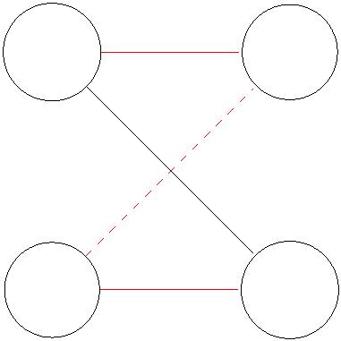
To efficiently search for such a path, let’s just follow our nose. It turns out that breadth-
first search (BFS), with a twist to enforce M-alternation, is all we need.
6
5
1
2
3
4
8
7
Figure 7: Dashed edges are the edges in the matching. Only tight edges are shown.
The algorithm will be clear from an example. Consider the graph in Figure 7; only the
tight edges are shown. Note that the graph does not contain a good path (if it did, we
could use it to augment the current matching to obtain a perfect matching, but vertex #4 is
isolated so there is no perfect matching.).2 So we know in advance that our search will fail.
But it’s useful to see what happens when it fails.
2
1
5
6
3
7
8
Figure 8: BFS spanning tree if we start BFS travel from node 3. Note that the edge {2, 6}
is not used.
We start a graph search from an unmatched vertex of V (the first such vertex, say); see
also Figure 8. In the example, this is vertex #3. Layer 0 of our search tree is {3}. We
obtain layer 1 from layer 0 by BFS; thus, layer 1 is {2, 7}. Note that if either 2 or 7 is
unmatched, then we have found a (one-hop) good path and we can stop the search. Both 2
and 7 are already matched in the example, however. Here is the twist to BFS: at the next
layer 2 we put only the vertices to which 2 and 7 are matched, namely 1 and 8. Conspicuous
in its absence is vertex #6; in regular BFS it would be included in layer 2, but here we
omit it because it is not matched to a vertex of layer 1. The reason for this twist is that
we want every path in our search tree to be M-alternating (since good paths need to be
M-alternating).
2
Remember we assume only that G contains a perfect matching; the subgraph of tight edges at any given
time will generally not contain a perfect matching.
9
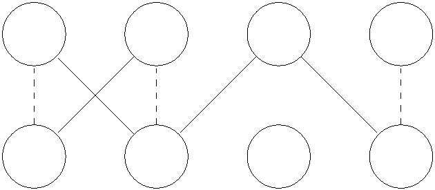
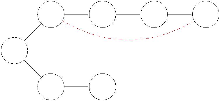

We then switch back to BFS. At vertex #8 we’re stuck (we’ve already seen its only
neighbor, #7). At vertex #1, we’ve already seen its neighbor 2 but have not yet seen vertex
#
5, so the third layer is {5}. Note that if 5 were unmatched, we would have found a good
path, from 5 back to the root 3. (All edges in the tree are tight by definition; the path is
alternating and of odd length, joining two unmatched vertices of V and W.) But 5 is already
matched to 6, so layer 4 of the search tree is {6}. We’ve already seen both of 6’s neighbors
before, so at this point we’re stuck and the search terminates.
In general, here is the search procedure for finding a good path (given a current match-
ing M and prices p).
Searching for a Good Path
level 0 = the first unmatched vertex r of V
while not stuck and no other unmatched vertex found do
if next level i is odd then
define level i from level i − 1 via BFS
/
/ i.e., neighbors of level i − 1 not already seen
else if next level i is even then
define level i as the vertices matched in M to vertices at
level i − 1
if found another unmatched vertex w then
return the search tree path between the root r and w
else
return “stuck”
To understand this subroutine, consider an edge (v, w) ∈ M, and suppose that v is
reached first, at level i. Importantly, it is not possible that w is also reached at level i. This
is where we use the assumption that G is bipartite: if v, w are reached in the same level,
then pasting together the paths from r to v and from r to w (which have the same length)
with the edge (v, w) exhibits an odd cycle, contradicting bipartiteness. Second, we claim
that i must be odd (cf., Figure 8). The reason is just that, by construction, every vertex
at an even level (other than 0) is the second endpoint reached of some matched edge (and
hence cannot be the endpoint of any other matched edge). We conclude that:
(*) if either endpoint of an edge of M is reached in the search tree, then both endpoints
are reached, and they appear at consecutive levels i, i + 1 with i odd.
Suppose the search tree reaches an unmatched vertex w other than the root r. Since
every vertex at an even level (after 0) is matched to a vertex at the previous level, w must
be at an odd level (and hence in W). By construction, every edge of the search tree is tight,
and every path in the tree is M-alternating. Thus the r-w path in the search tree is a good
path, allowing us to increase the size of M by 1.
1
0

4
.4 Good Sets
Suppose the search gets stuck, as in our example. How do we make progress, and in what
sense? In this case, we keep the matching the same but update the prices.
Define S ⊆ V as the vertices at even levels. Define N(S) ⊆ S as the neighbors of S via
tight edges, i.e.,
N(S) = {w : ∃v ∈ S with (v, w) tight}.
(4)
We claim that N(S) is precisely the vertices that appear in the odd levels of the search tree.
In proof, first note that every vertex at an odd level is (by construction/BFS) adjacent via a
tight edge to a vertex at the previous (even) level. For the converse, every vertex w ∈ N(S)
must be reached in the search, because (by basic properties of graph search) the search can
only stuck if there are no unexplored edges out of any even vertex.
The set S is a good set, in that is satisfies:
1
2
. S contains an unmatched vertex;
. every vertex of N(S) is matched in M to a vertex of S (since the search failed, every
vertex in an odd level is matched to some vertex at the next (even) level).
See also Figure 9.
1
2
3
5
4
6
7
Figure 9: S = {1, 2, 3, 4} is example of good set, with N(S) = {5, 6}. Only black edges are
tight edges (i.e. (4, 7) is not tight). The matching edges are dashed.
Having found such a good set S, the Hungarian algorithm updates prices as follows.
Price Update Step
given a good set S, with neighbors via tight edges N(S)
for all v ∈ S do
increase p by ∆
v
for all w ∈ N(S) do
decrease p by ∆
v
/ ∆ is as large as possible, subject to invariants
/
1
1
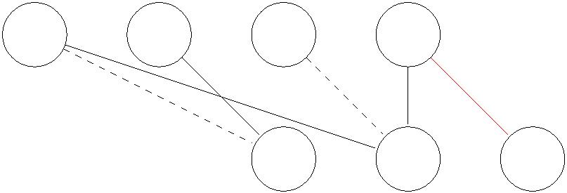

Prices in S (on the left-hand side) are increased, while prices in N(S) (on the right-hand
side) are decreased by the same amount. How does this affect the reduced cost of each edge
of G (Figure 9)?
1
2
3
4
. for an edge (v, w) with v ∈/ S and w ∈/ N(S), the prices of v, w are unchanged so cp
vw
is unchanged;
. for an edge (v, w) with v ∈ S and w ∈ N(S), the sum of the prices of v, w is unchanged
(one increased by ∆, the other decreased by ∆) so cp is unchanged;
vw
. for an edge (v, w) with v ∈/ S and w ∈ N(S), p stays the same while p goes down by
v
w
∆
, so cp goes up by ∆;
vw
. for an edge (v, w) with v ∈ S and w ∈/ N(S), p stays the same while p goes up by
w
v
∆
, so cp goes down by ∆.
vw
So what happens with the invariants? Recalling (*) from Section 4.3, we see that edges of M
are in either the first or second category. Thus they stay tight, and the second invariant
remains satisfied. The first invariant is endangered by edges in the fourth category, whose
reduced costs are dropping with ∆.3 By the definition of N(S), edges in this category are
not tight. So we increase ∆ to the largest-possible value subject to the first invariant — the
first point at which the reduced cost of some edge in the fourth category is zeroed out.4
Every price update makes progress, in the sense that it strictly increases the size of search
tree. To see this, suppose a price update causes the edge (v, w) to become tight (with v ∈ S,
w ∈/ N(S)). What happens in the next iteration, when we search from the same vertex r
for a good path? All edges in the previous search tree fall in the second category, and hence
are again tight in the next iteration. Thus, the search procedure will regrow exactly the
same search tree as before, will again reach the vertex v, and now will also explore along the
newly tight edge (v, w), which adds the additional vertex w ∈ W to the tree. This can only
happen n times in a row before finding a good path, since there are only n vertices in W.
3
Edges in third category might go from tight to non-tight, but these edges are not in M (every vertex of
N(S) is matched to a vertex of S) and so no invariant is violated.
A detail: how do we know that such an edge exists? If not, then all neighbors of S in G (via tight edges
4
or not) belong to N(S). The two properties of good sets imply that |N(S)| < |S|. But this violates Hall’s
condition for perfect matchings (Lecture #4), contradicting our standing assumption that G has at least one
perfect matching.
1
2

4
.5 The Hungarian Algorithm (All in One Place)
The Hungarian Algorithm
set M = ∅
set p = 0 for all v ∈ V ∪ W
v
while M is not a perfect matching do
level 0 of search tree T = the first unmatched vertex r of V
while not stuck and no other unmatched vertex found do
if next level i is odd then
define level i of T from level i − 1 via BFS
/
/ i.e., neighbors of level i − 1 not already seen
else if next level i is even then
define level i of T as the vertices matched in M to vertices at
level i − 1
if T contains an unmatched vertex w ∈ W then
let P denote the r-w path in T
replace M by M ⊕ P
else
let S denote the vertices of T in even levels
let N(S) denote the vertices of T in odd levels
for all v ∈ S do
increase p by ∆
v
for all w ∈ N(S) do
decrease p by ∆
v
/ ∆ is as large as possible, subject to invariants
/
return M
4
.6 Running Time
Since M can only contain n edges, there can only be n iterations that find a good path.
Since the search tree can only contain n vertices of W, there can only be n prices updates
between iterations that find good paths. Computing the search tree (and hence P or S and
N(S)) and ∆ (if necessary) can be done in O(m) time. This gives a running time bound of
O(mn2). See Problem Set #2 for an implementation with running time O(mn log n).
4
.7 Example
We reinforce the algorithm via an example. Consider the graph in Figure 10.
1
3

2
7
v(0)
x(0)
w(0)
y(0)
5
3
Figure 10: Example graph. Initially, all prices are 0.
We initialize all prices to 0 and the current matching to the empty set. Initially, there
are no tight edges, so there is certainly no good path. The search for such a path gets stuck
where it starts, at vertex v. So S = {v} and N(S) = ∅. We execute a price update step,
raising the price of v to 2, at which point the edge (v, w) becomes tight. Next iteration,
the search starts at v, explores the tight edge (v, w), and encounters vertex w, which is
unmatched. Thus this edge is added to the current matching. Next iteration, a new search
starts from the only remaining unmatched vertex on the left (x). It has no tight incident
edges, so the search gets stuck immediately, with S = {x} and N(S) = ∅. We thus do a price
update step, with ∆ = 5, at which point the edge (x, w) becomes newly tight. Note that
the edges (v, y) and (x, y) have reduced costs 1 and 2, respectively, so neither is tight. Next
iteration, the search from x explores the incident tight edge (x, w). If w were unmatched,
we could stop the search and add the edge (x, w). But w is already matched, to v, so w and
v are placed at levels 1 and 2 of the search tree. v has no tight incident edges other than
to w, so the search gets stuck here, with S = {x, v} and N(S) = {w}. So we do another a
price update step, increasing the price of x and v by ∆ and decreasing the price of w by ∆.
With ∆ = 1, the reduced cost of edge (v, y) gets zeroed out. The final iteration discovers
the good path x → w → v → y. Augmenting on this path yields the minimum-cost perfect
matching {(v, y), (x, w)}.
1
4
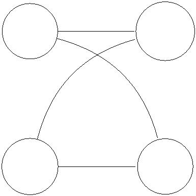
CS261: A Second Course in Algorithms
Lecture #6: Generalizations of Maximum Flow and
Bipartite Matching∗
Tim Roughgarden†
January 21, 2016
1
Fundamental Problems in Combinatorial Optimiza-
tion
Figure 1: Web of six fundamental problems in combinatorial optimization. The ones covered
thus far are in red. Each arrow points from a problem to a generalization of that problem.
We started the course by studying the maximum flow problem and the closely related s-t
cut problem. We observed (Lecture #4) that the maximum-cardinality bipartite matching
∗
†
ꢀc
2
Department of Computer Science, Stanford University, 474 Gates Building, 353 Serra Mall, Stanford,
016, Tim Roughgarden.
CA 94305. Email: tim@cs.stanford.edu.
1
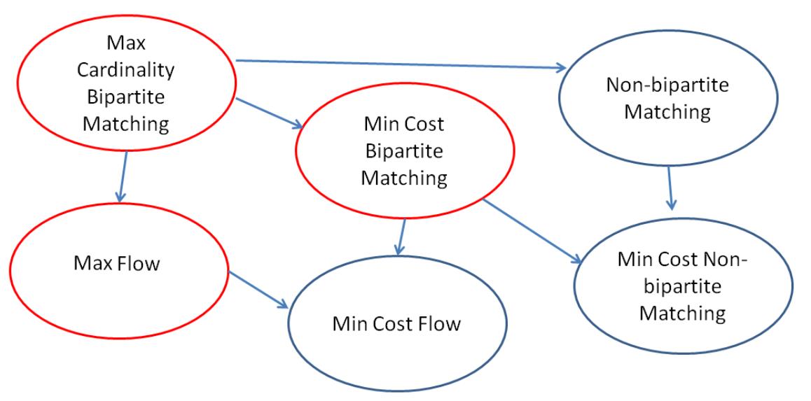

problem can be viewed as a special case of the maximum flow problem (Figure 1). We
then generalized the former problem to include edge costs, which seemed to give a problem
incomparable to maximum flow.
The inquisitive student might be wondering the following:
1
. Is there a natural common generalization of the maximum flow and minimum-cost
bipartite matching problems?
2
. What’s up with graph matching in non-bipartite graphs?
The answer to the first question is “yes,” and it’s a problem known as minimum-cost flow
(Figure 1). For the second question, there is a nice theory of graph matchings in non-
bipartite graphs, both for the maximum-cardinality and minimum-cost cases, although the
theory is more difficult and the algorithms are slower than in the bipartite case. This lecture
introduces the three new problems in Figure 1 and some essential facts you should know
about them. The six problems in Figure 1, along with the minimum spanning tree and
shortest path problems that you already know well from CS161, arguably form the complete
list of the most fundamental problems in combinatorial optimization, the study of efficiently
optimizing over large collections of discrete structures.
The main take-ways from this lecture’s high-level discussion are:
1
. You should know about the existence of the minimum-cost flow and non-bipartite
matching problems. They do come up in applications, if somewhat less frequently
than the problems studied in the first five lectures.
2
. There are reasonably efficient algorithms for all of these problems, if a bit slower than
the state-of-the-art algorithms for the problems discussed previously. We won’t discuss
running times in any detail, but think of roughly O(mn) or O(n3) as a typical time
bound of a smart algorithm for these problems.
3
. The algorithms and analysis for these problems follow exactly the same principles that
you’ve been studying in previous lectures. They use optimality conditions, various
progress measures, well-chosen invariants, and so on. So you’re well-positioned to
study deeply these problems and algorithms for them, in another course or on your own.
Indeed, if CS261 were a semester-long course, we would cover this material in detail
over the next 4-5 lectures. (Alas, it will be time to move on to linear programming.)
2
The Minimum Cost Flow Problem
An instance of the minimum-cost flow problem consists of the following ingredients:
•
•
a directed graph G = (V, E);
a source s ∈ V and sink t ∈ V ;
2
•
•
•
a target flow value d;
a nonnegative capacity ue for each edge e ∈ E;
a real-valued cost ce for each edge e ∈ E.
The goal is to compute a flow f with value d — that is, pushing d units of flow from s to
t, subject to the usual conservation and capacity constraints — that minimizes the overall
cost
X
c f .
e
(1)
e
e∈E
Note that, for each edge e, we think of c as a “per-flow unit” cost, so with f units of flow
e
e
the contribution of edge e to the overall cost is c f .1
e
e
There are two differences with the maximum flow problem. The important one is that
now every edge has a cost. (In maximum flow, one can think of all the costs being 0.) The
second difference, which is artificial, is that we specified a specific amount of flow d to send.
There are multiple other equivalent formulations of the minimum-cost flow problem. For
example, one can ask for the maximum flow with the minimum cost. Alternatively, instead
of having a source s and sink t, one can ask for a “circulation” — meaning a flow that
satisfies conservation constraints at every vertex of V — with the minimum cost (in the
sense of (1)).2
Impressively, the minimum-cost flow problem captures three different problems that
you’ve studied as special cases.
1
. Shortest paths. Suppose you are given a “black box” that quickly does minimum-
cost flow computations, and you want to compute the shortest path between some s
and some t is a directed graph with edge costs. The black box is expecting a flow
value d and edge capacities ue (in addition to G, s, t, and the edge costs); we just
set d = 1 and ue = 1 (say) for every edge e. An integral minimum-cost flow in this
network will be a shortest path from s to t (why?).
2
3
. Maximum flow. Given an instances of the maximum flow problem, we need to define
d and edge costs before feeding the input into our minimum-cost flow black box. The
edge costs should presumably be set to 0. Then, to compute the maximum flow value,
we can just use binary search to find the largest value of d for which the black box
returns a feasible solution.
. Minimum-cost perfect bipartite matching. The reduction here is the same as
that from maximum-cardinality bipartite matching to maximum flow (Lecture #4) —
the edge costs just carry over. The value d should be set to n, the number of vertices
on each side of the bipartite graph (why?).
1
If there is no flow of value d, then an algorithm should report this fact. Note this is easy to check with
a single maximum flow computation.
Of course if all edge costs are nonnegative, then the all-zero solution is optimal. But with negative
cycles, this is a nontrivial problem.
2
3

Problem Set #2 explores various aspects of minimum-cost flows. Like the other prob-
lems we’ve studied, there are nice optimality conditions for minimum-cost flows. First, one
extends the notion of a residual network to networks with costs — the only twist is that
if an edge (w, v) of the residual network is the reverse edge corresponding to (v, w) ∈ E,
then the cost of cwv should be set to −c . (Which makes sense given that reverse edges
vw
correspond to “undo” operations.) Then, a flow with value d is minimum-cost if and only
if the corresponding residual network has no negative cycle. This then suggests a simple
“
cycle-canceling” algorithm, analogous to the Ford-Fulkerson algorithm. Polynomial-time
algorithms can be designed using the same ideas we used for maximum flow in Lectures
2 and #3 and Problem Set #1 (blocking flows, push-relabel, scaling, etc.). There are
#
algorithms along these lines with running time roughly O(mn) that are also quite fast in
practice. (Theoretically, it is also known how do a bit better.) In general, you should be
happy if a problem that you care about reduces to the minimum-cost flow problem.
3
Non-Bipartite Matching
3
.1 Maximum-Cardinality Non-Bipartite Matching
In the general (non-bipartite) matching problem, the input is an undirected graph G =
(V, E), not necessarily bipartite. The goal to compute a matching (as before, a subset
M ⊆ E with no shared endpoints) with the largest cardinality. Recall that the simplest
non-bipartite graphs are odd cycles (Figure 2).
b
d
a
c
e
Figure 2: Example of non-bipartite graph: odd cycle.
A priori, it is far from obvious that the general graph matching problem is solvable in
polynomial time (as opposed to being NP-hard). It appears to be significantly more difficult
than the special case of bipartite matching. For example, there does not seem to be a natural
reduction from non-bipartite matching to the maximum flow problem. Once again, we need
to develop from scratch algorithms and strategies for correctness,
The non-bipartite matching problem admits some remarkable optimality conditions. For
motivation, what is the maximum size of a matching in the graph in Figure 3? There are 16
4
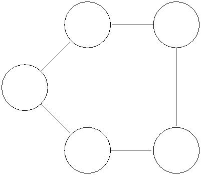
vertices, so clearly a matching has at most 8 edges. It’s easy to exhibit a matching of size 6
(Figure 3), but can we do better?
1
6
2
3
5
7
9
8
4
11
12
1
0
14
13
1
5
16
Figure 3: Example graph. A matching of size 6 is denoted by dashed edges.
Here’s one way to argue that there is no better matching. In each of the 5 triangles, at
most 2 of the 3 vertices can be matched to each other. This leaves at least five vertices,
one from each triangle, that, if matched, can only be matched to the center vertex. The
center vertex can only be matched to one of these five, so every matching leaves at least four
vertices unmatched. This translates to matching at most 12 vertices, and hence containing
at most 6 edges.
In general, we have the following.
Lemma 3.1 In every graph G = (V, E), the maximum cardinality of a matching is at most
1
min [|V | − (oc(S) − |S|)] ,
(2)
2
S⊆V
where oc(S) denotes the number of odd-size connected components in the graph G \ S.
Note that G\S consists of the pieces left over after ripping the vertices in S out of the graph
G (Figure 4).
5
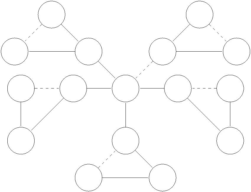

Figure 4: Suppose removing S results in 4 connected components, A, B, C and D. If 3 of
them are odd-sized, then oc(S) = 3
For example, in the Figure 3, we effectively took S to be the center vertex, so oc(S) = 5
1
(since G\S is the five triangles) and (2) is (16 (5 1)) = 6. The proof is a straightforward
−
−
2
generalization of our earlier argument.
Proof of Lemma 3.1: Fix S ⊆ V . For every odd-size connected component C of G \ S,
at least one vertex of C is not matched to some other vertex of C. These oc(S) vertices
can only be matched to vertices of S (if two vertices of C and C could be matched to
1
2
each other, then C and C would not be separate connected components of G \ S). Thus,
1
2
every matching leaves at least oc(S) − |S| vertices unmatched, and hence matches at most
|
V | − (oc(S) − |S|) vertices, and hence has at most 1(|V | − (oc(S) − |S|)) edges. Ranging
2
over all choices of S ⊆ V yields the upper bound in (2). ꢀ
Lemma 3.1 is an analog of the fact that a maximum flow is at most the value of a
minimum s-t cut. We can think of (2) as the best upper bound that we can prove if we
restrict ourselves to “obvious obstructions” to large matchings. Certainly, if we ever find a
matching with size equal to (2), then no other matching could be bigger. But can there be a
gap between the maximum size of a matching and the upper bound in (2)? Could there be
obstructions to large matchings more subtle than the simple parity argument used to prove
Lemma 3.1? One of the more beautiful theorems in combinatorics asserts that there can
never be a gap.
Theorem 3.2 (Tutte-Berge Formula) In Lemma 3.1, equality always holds:
1
max matching size = min [|V | − (oc(S) − |S|)] .
2
S⊆V
The original proof of the Tutte-Berge formula is via induction, and does not seems to lead
to an efficient algorithm.3 In 1965, Edmonds gave the first polynomial-time algorithm for
3
Tutte characterized the graphs with perfect matchings in the 1940s; in the 1950s, Berge extended this
characterization to prove Theorem 3.2.
6
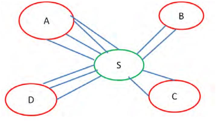


computing a maximum-cardinality matching.4 Since the algorithm is guaranteed to produce
a matching with cardinality equal to (2), Edmonds’ algorithm provides an algorithmic proof
of the Tutte-Berge formula.
A key challenge in non-bipartite matching is searching for a good path to use to increase
the size of the current matching. Recall that in the Hungarian algorithm (Lecture #5), we
used the bipartite assumption to argue that there’s no way to encounter both endpoints of
an edge in the current matching in the same level of the search tree. But this certainly can
happen in non-bipartite graphs, even just in the triangle. Edmonds called these odd cycles
“
blossoms,” and his algorithm is often called the “blossom algorithm.” When a blossom is
encountered, it’s not clear how to proceed with the search. Edmonds’ idea was to “shrink,”
meaning contract, a blossom when one is found. The blossom becomes a super-vertex in
the new (smaller) graph, and the algorithm can continue. All blossoms are uncontracted in
reverse order at the end of the algorithm.5
3
.2 Minimum-Cost Non-Bipartite Matching
An algorithm designer is never satisfied, always wanting better and more general solutions
to computational problems. So it’s natural to consider the graph matching problem with
both of the complications that we’ve studied so far: general (non-bipartite) graphs and edge
costs.
The minimum-cost non-bipartite matching problem is again polynomial-time solvable,
again first proved by Edmonds. From 30,000 feet, the idea to combine the blossom shrinking
idea above (which handles non-bipartiteness) with the vertex prices we used in Lecture #5
for the Hungarian algorithm (which handle costs). This is not as easy as it sounds, however
— it’s not clear what prices should be given to super-vertices when they are created, and
such super-vertices may need to be uncontracted mid-algorithm. With some care, however,
this idea can be made to work and yields a polynomial-time algorithm.
While polynomial-time solvable, the minimum-cost matching problem is a relatively hard
problem within the class P. State-of-the-art algorithms can handle graphs with 100s of
vertices, but graphs with 1000s of vertices are already a challenge. From your other computer
science courses, you know that in applications one often wants to handle graphs that are
bigger than this by 1–6 orders of magnitude. This motivates the design of heuristics for
matching that are very fast, even if not fully correct.6
For example, the following Kruskal-like greedy algorithm is a natural one to try. For
convenience, we work with the equivalent maximum-weight version of the problem (each edge
4
In this remarkable paper, titled “Paths, Trees, and Flowers,” Edmonds defines the class of polynomial-
time solvable problems and conjectures that the traveling salesman problem is not in the class (i.e., that
P = NP). Keep in mind that NP-completeness wasn’t defined (by Cook and Levin) until 1971.
5
Your instructor covered this algorithm in last year’s CS261, in honor of the algorithm’s 50th anniversary.
It takes two lectures, however, and has been cut this year in favor of other topics.
In the last part of the course, we explore this idea in the context of approximation algorithms for
6
NP-hard problems. It’s worth remembering that for sufficiently large data sets, approximation is the most
appropriate solution even for problems that are polynomial-time solvable.
7

has a weight we, the goal is to compute the matching with largest sum of weights).
Greedy Matching Algorithm
sort and rename the edges E = {1, 2, . . . , m} so that w ≥ w ≥ · · · w
1
2
m
M = ∅
for i = 1 to m do
if ei shares no endpoint with edges in M then
add ei to M
1
1+ꢀ
1
a
c
b
d
Figure 5: The greedy algorithm picks the edge (b, c), while the optimal matching consists of
(a, b) and (c, d).
A simple example (Figure 5) shows that, at least for some graphs, the greedy algorithm
can produce a matching with weight only 50% of the maximum possible. On Problem Set
#
2 you will prove that there are no worse examples — for every (non-bipartite) graph and
edge weights, the matching output by the greedy algorithm has weight at least 50% of the
maximum possible. Just over the past few years, new matching approximation algorithms
have been developed, and it’s now possible to get a (1 − ꢀ)-approximation in O(m) time, for
1
any constant ꢀ > 0 (the hidden constant in the “big-oh” depends on ) [?].
ꢀ
8

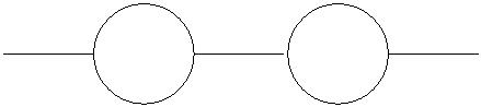

CS261: A Second Course in Algorithms
Lecture #7: Linear Programming: Introduction and
Applications∗
Tim Roughgarden†
January 26, 2016
1
Preamble
With this lecture we commence the second part of the course, on linear programming, with
an emphasis on applications on duality theory.1 We’ll spend a fair amount of quality time
with linear programs for two reasons.
First, linear programming is very useful algorithmically, both for proving theorems and
for solving real-world problems.
Linear programming is a remarkable sweet spot between power/generality and
computational efficiency.
For example, all of the problems studied in previous lectures can be viewed as special cases
of linear programming, and there are also zillions of other examples. Despite this generality,
linear programs can be solved efficiently, both in theory (meaning in polynomial time) and
in practice (with input sizes up into the millions).
Even when a computational problem that you care about does not reduce directly to
solving a linear program, linear programming is an extremely helpful subroutine to have in
your pocket. For example, in the fourth and last part of the course, we’ll design approx-
imation algorithms for NP-hard problems that use linear programming in the algorithm
and/or analysis. In practice, probably most of the cycles spent on solving linear programs
is in service of solving integer programs (which are generally NP-hard). State-of-the-art
∗
†
ꢀc
2
Department of Computer Science, Stanford University, 474 Gates Building, 353 Serra Mall, Stanford,
016, Tim Roughgarden.
CA 94305. Email: tim@cs.stanford.edu.
The term “programming” here is not meant in the same sense as computer programming (linear program-
1
ming pre-dates modern computers). It’s in the same spirit as “television programming,” meaning assembling
a scheduled of planned activities. (See also “dynamic programming”.)
1

algorithms for the latter problem invoke a linear programming solver over and over again to
make consistent progress.
Second, linear programming is conceptually useful —- understanding it, and especially
LP duality, gives you the “right way” to think about a host of different problems in a simple
and consistent way. For example, the optimality conditions we’ve studied in past lectures
(like the max-flow/min-cut theorem and Hall’s theorem) can be viewed as special cases of
linear programming duality. LP duality is more or less the ultimate answer to the question
“how do we know when we’re done?” As such, it’s extremely useful for proving that an
algorithm is correct (or approximately correct).
We’ll talk about both these aspects of linear programming at length.
2
How to Think About Linear Programming
2
.1 Comparison to Systems of Linear Equations
Once upon a time, in some course you may have forgotten, you learned about linear systems
of equations. Such a system consists of m linear equations in real-valued variables x , . . . , x :
1
n
a x + a x + · · · + a x = b
1
1
1
12
2
1n
n
1
2
a x + a x + · · · + a x = b
2
1
1
22
2
2n
n
.
.
.
.
.
.
a x + a x + · · · + a x = b .
m1
1
m2
2
mn
n
m
The a ’s and the b ’s are given; the goal is to check whether or not there are values for the
ij
i
xj’s such that all m constraints are satisfied. You learned at some point that this problem
can be solved efficiently, for example by Gaussian elimination. By “solved” we mean that
the algorithm returns a feasible solution, or correctly reports that no feasible solution exists.
Here’s an issue, though: what about inequalities? For example, recall the maximum flow
problem. There are conservation constraints, which are equations and hence OK. But the
capacity constraints are fundamentally inequalities. (There is also the constraint that flow
values should be nonnegative.) Inequalities are part of the problem description of many
other problems that we’d like to solve. The point of linear programming is to solve systems
of linear equations and inequalities. Moreover, when there are multiple feasible solutions, we
would like to compute the “best” one.
2
.2 Ingredients of a Linear Program
There is a convenient and flexible language for specifying linear programs, and we’ll get lots
of practice using it during this lecture. Sometimes it’s easy to translate a computational
problem into this language, sometimes it takes some tricks (we’ll see examples of both).
To specify a linear program, you need to declare what’s allowed and what you want.
2
Ingredients of a Linear Program
. Decision variables x , . . . , x ∈ R.
1
2
1
n
. Linear constraints, each of the form
Xn
ajxj (∗) bi,
j=1
where (*) could be ≤, ≥, or =.
. A linear objective function, of the form
Xn
3
max
min
cjxj
j=1
or
Xn
c x .
j
j
j=1
Several comments. First, the a ’s, b ’s, and c ’s are constants, meaning they are part of the
i
ij
j
input, numbers hard-wired into the linear program (like 5, -1, 10, etc.). The xj’s are free, and
it is the job of a linear programming algorithm to figure out the best values for them. Second,
when specifying constraints, there is no need to make use of both “≤” and “≥”inequalities
—
one can be transformed into the other just by multiplying all the coefficients by -1 (the
a ’s and b ’s are allowed to be positive or negative). Similarly, equality constraints are
ij
i
superfluous, in that the constraint that a quantity equals bi is equivalent to the pair of
inequality constraints stating that the quantity is both at least b and at most b . Finally,
i
there is also no difference between the “min” and “max” cases for the objective function
i
—
allowed to be positive or negative).
one is easily converted into the other just by multiplying all the c ’s by -1 (the c ’s are
j
j
So what’s not allowed in a linear program? Terms like x2, x x , log(1 + x ), etc. So
j
j
k
j
whenever a decision variable appears in an expression, it is alone, possibly multiplied by
a constant (and then summed with other such terms). While these linearity requirements
may seem restrictive, we’ll see that many real-world problems can be formulated as or well
approximated by linear programs.
3

2
.3 A Simple Example
Figure 1: a toy example of linear program.
To make linear programs more concrete and develop your geometric intuition about them,
let’s look at a toy example. (Many “real” examples of linear programs are coming shortly.)
Suppose there are two decision variables x and x — so we can visualize solutions as
1
2
points (x , x ) in the plane. See Figure 2.3. Let’s consider the (linear) objective function of
1
maximizing the sum of the decision variables:
2
max x + x .
1
2
We’ll look at four (linear) constraints:
x1 ≥ 0
x2 ≥ 0
2
x1 + x2 ≤ 1
x1 + 2x2 ≤ 1.
The first two inequalities restrict feasible solutions to the non-negative quadrant of the
plane. The second two inequalities further restrict feasible solutions to lie in the shaded
region depicted in Figure 2.3. Geometrically, the objective function asks for the feasible
point furthest in the direction of the coefficient vector (1, 1) — the “most northeastern”
feasible point. Put differently, the level sets of the objective function are parallel lines
running northwest to southeast.2 Eyeballing the feasible region, this point is ( , ), for an
1
1
3
optimal objective function value of . This is the “last point of intersection” between a
3
2
3
level set of the objective function and the feasible region (as one sweeps from southwest to
northeast).
2
Recall that a level set of a function g has the form {x : g(x) = c}, for some constant c. That is, all
points in a level set have equal objective function value.
4
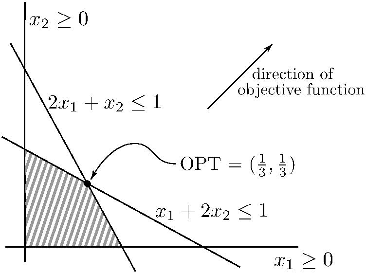


2
.4 Geometric Intuition
While it’s always dangerous to extrapolate from two or three dimensions to an arbitrary
number, the geometric intuition above remains valid for general linear programs, with an ar-
bitrary number of dimensions (i.e., decision variables) and constraints. Even though we can’t
draw pictures when there are many dimensions, the relevant algebra carries over without any
difficulties. Specifically:
1
2
3
. A linear constraint in n dimensions corresponds to a halfspace in Rn. Thus a feasible
region is an intersection of halfspaces, the higher-dimensional analog of a polygon.3
. The level sets of the objective function are parallel (n − 1)-dimensional hyperplanes in
Rn, each orthogonal to the coefficient vector c of the objective function.
. The optimal solution is the feasible point furthest in the direction of c (for a maximiza-
tion problem) or −c (for a minimization problem). Equivalently, it is the last point of
intersection (traveling in the direction c or −c) of a level set of the objective function
and the feasible region.
4
. When there is a unique optimal solution, it is a vertex (i.e., “corner”) of the feasible
region.
There are a few edge cases which can occur but are not especially important in CS261.
1
. There might be no feasible solutions at all. For example, if we add the constraint
x + x ≥ 1 to our toy example, then there are no longer any feasible solutions. Linear
1
programming algorithms correctly detect when this case occurs.
2
2
3
. The optimal objective function value is unbounded (+∞ for a maximization problem,
−
∞ for a minimization problem). Note a necessary but not sufficient condition for
this case is that the feasible region is unbounded. For example, if we dropped the
constraints 2x + x ≤ 1 and x + 2x ≤ 1 from our toy example, then it would have
1
2
1
2
unbounded objective function value. Again, linear programming algorithms correctly
detect when this case occurs.
. The optimal solution need not be unique, as a “side” of the feasible region might
be parallel to the levels sets of the objective function. Whenever the feasible region
is bounded, however, there always exists an optimal solution that is a vertex of the
feasible region.4
3
A finite intersection of halfspaces is also called a “polyhedron;” in the common special case where the
feasible region is bounded, it is called a “polytope.”
There are some annoying edge cases for unbounded feasible regions, for example the linear program
max(x + x ) subject to x + x = 1.
4
1
2
1
2
5

3
Some Applications of Linear Programming
Zillions of problems reduce to linear programming. It would take an entire course to cover
even just its most famous applications. Some of these applications are conceptually a bit
boring but still very important — as early as the 1940s, the military was using linear pro-
gramming to figure out the most efficient way to ship supplies from factories to where they
were needed.5 Several central problems in computer science reduce to linear programming,
and we describe some of these in detail in this section. Throughout, keep in mind that all
of these linear programs can be solved efficiently, both in theory and in practice. We’ll say
more about algorithms for linear programming in a later lecture.
3
.1 Maximum Flow
If we return to the definition of the maximum flow problem in Lecture #1, we see that it
translates quite directly to a linear program.
1
. Decision variables: what are we try to solve for? A flow, of course, Specifically, the
amount f of flow on each edge e. So our variables are just {f }e∈E.
. Constraints: Recall we have conservation constraints and capacity constraints. We
e
e
2
can write the former as
X
X
fe −
{z } | {z }
fe = 0
e∈δ−(v)
e∈δ−(v)
|
flow in
flow out
for every vertex v = s, t.6 We can write the latter as
fe ≤ ue
for every edge e ∈ E. Since decision variables of linear programs are by default allowed
to take on arbitrary real values (positive or negative), we also need to remember to
add nonnegativity constraints:
fe ≥ 0
for every edge e ∈ E. Observe that every one of these 2m + n − 2 constraints (where
m = |E| and n = |V |) is linear — each decision variable f only appears by itself (with
e
a coefficient of 1 or -1).
3
. Objective function: We just copy the same one we used in Lecture #1:
X
max
f .
e
e∈δ+(s)
Note that this is again a linear function.
5
Note this is well before computer science was field; for example, Stanford’s Computer Science Department
was founded only in 1965.
6
Recall that δ− and δ+ denote the edges incoming to and outgoing from v, respectively.
6


3
.2 Minimum-Cost Flow
In Lecture #6 we introduced the minimum-cost flow problem. Extending specialized al-
gorithms for maximum flow to generalized algorithms takes non-trivial work (see Problem
Set #2 for starters). If we’re just using linear programming, however, the generalization
is immediate.7 The main change is in the objective function. As defined last lecture, it is
simply
X
min
c f ,
e
e
e∈E
where c is the cost of edge e. Since the c ’s are fixed numbers (i.e., part of the input), this
e
is a linear objective function.
e
For the version of the minimum-cost flow problem defined last lecture, we should also
add the constraint
X
fe = d,
e∈δ+(s)
where d is the target flow value. (One can also add the analogous constraint for t, but this
is already implied by the other constraints.)
To further highlight how flexible linear programs can be, suppose we want to impose a
lower bound `e (other than 0) on the amount of flow on each edge e, in addition to the
usual upper bound ue. This is trivial to accommodate in our linear program — just replace
“
f ≥ 0” by f ≥ ` .8
e
e
e
3
.3 Fitting a Line
We now consider two less obvious applications of linear programming, to basic problems in
machine learning. We first consider the problem of fitting a line to data points (i.e., linear
regression), perhaps the simplest non-trivial machine learning problem.
Formally, the input consists of m data points p1, . . . , pm ∈ Rd, each with d real-valued
“
features” (i.e., coordinates).9 For example, perhaps d = 3, and each data point corresponds
to a 3rd-grader, listing the household income, number of owned books, and number of years
of parental education. Also part of the input is a “label” ` ∈ R for each point pi.10 For
i
example, ` could be the score earned by the 3rd-grader in question on a standardized test.
i
We reiterate that the pi’s and `i’s are fixed (part of the input), not decision variables.
7
While linear programming is a reasonable way to solve the maximum flow and minimum-cost flow
problems, especially if the goal is to have a “quick and dirty” solution, but the best specialized algorithms
for these problems are generally faster.
8
If you prefer to use flow algorithms, there is a simple reduction from this problem to the special case
with ` = 0 for all e ∈ E (do you see it?).
e
Feel free to take d = 1 throughout the rest of the lecture, which is already a practically relevant and
9
computationally interesting case.
0This is a canonical “supervised learning” problem, meaning that the algorithm is provided with labeled
data.
1
7

Informally, the goal is to expresses the `i as well as possible as a linear function of the
p ’s. That is, the goal is to compute a linear function h : Rd → R such that h(pi) ≈ ` for
i
every data point i.
i
The two most common motivations for computing a “best-fit” linear function are pre-
diction and data analysis. In the first scenario, one uses labeled data to identify a linear
function h that, at least for these data points, does a good job of predicting the label `i
from the feature values pi. The hope is that this linear function “generalizes,” meaning that
it also makes accurate predictions for other data points for which the label is not already
known. There is a lot of beautiful and useful theory in statistics and machine learning about
when one can and cannot expect a hypothesis to generalize, which you’ll learn about if you
take courses in those areas. In the second scenario, the goal is to understand the relationship
between each feature of the data points and the labels, and also the relationships between
the different features. As a simple example, it’s clearly interesting to know when one of the d
features is much more strongly correlated with the label `i than any of the others.
We now show that computing the best line, for one definition of “best,” reduces to linear
programming. Recall that every linear function h : Rd → R has the form
Xd
for some coefficients a , . . . , a and intercept b. (This is one of several equivalent definitions
h(z) =
a z + b
j j
j=1
1
d
of a linear function.11 So it’s natural to take a , . . . , a , b as our decision variables.
1
d
What’s our objective function? Clearly if the data points are colinear we want to compute
the line that passes through all of them. But this will never happen, so we must compromise
between how well we approximate different points.
For a given choice of a , . . . , a , b, define the error on point i as
d
1
ꢀ
ꢀ
ꢀ
ꢀ
ꢀ
ꢀ
|
!
ꢀ
ꢀ
Xd
ꢀ
ꢀ
ꢀ
i
j
i
ꢀ
Ei(a, b) =
a p − b −
`
.
(1)
ꢀ
j
|{z}
ꢀ
ꢀ
ꢀ
j
−
1
“ground truth”
ꢀ
ꢀ
{z
}
ꢀ
ꢀ
prediction
Geometrically, when d = 1, we can think of each (pi, `i) as a point in the plane and (1) is
just the vertical distance between this point and the computed line.
In this lecture, we consider the objective function of minimizing the sum of errors:
Xm
This is not the most common objective for linear regression; more standard is minimizing the
min
a,b
Ei(a, b).
(2)
i=1
P
m
i=1
2
squared error
E (a, b). While our motivation for choosing (2) is primarily pedagogical,
i
1
1Sometimes people use “linear function” to mean the special case where b = 0, and “affine function” for
the case of arbitrary b.
8


this objective is reasonable and is sometimes used in practice. The advantage over squared
error is that it is more robust to outliers. Squaring the error of an outlier makes it a squeakier
wheel. That is, a stray point (e.g., a faulty sensor or data entry error) will influence the line
chosen under (2) less that it would with the squared error objective (Figure 2).12
Figure 2: When there exists an outlier (red point), using the objective function defined
in (2) causes the best-fit line not to ”stray” as far away from the non-outliers (blue line) as
when using the squared error objective (red line), because the squared error objective would
penalize more greatly when the chosen line is far from the outlier.
Consider the problem of choosing a, b to minimize (2). (Since the aj’s and b can be
anything, there are no constraints.) The problem: this is not a linear program. The source
of nonlinearity is the absolute value sign | · | in (1). Happily, in this case and many others,
absolute values can be made linear with a simple trick.
The trick is to introduce extra variables e , . . . , e , one per data point. The intent is for
1
m
e to take on the value E (a, b). Motivated by the identify |x| = max{x, −x}, we add two
i
constraints for each data point:
i
!
Xd
i
j
i
ei ≥
a p − b − `
(3)
(4)
j
j=1
and
"
!
#
Xd
i
i
ei ≥ −
a p − b − ` .
j
j
j=1
1
2Squared error can be minimized efficiently using an extension of linear programming known as convex
programming. (For the present “ordinary least squares” version of the problem, it can even be solved
analytically, in closed form.) We may discuss convex programming in a future lecture.
9
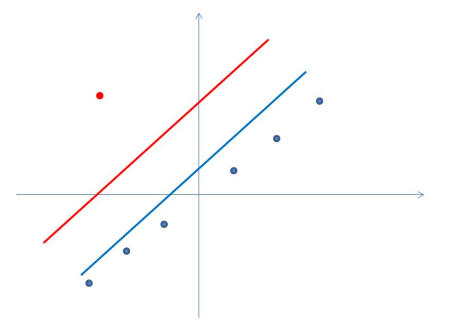

We change the objective function to
Xm
Note that optimizing (5) subject to all constraints of the form (3) and (4) is a linear program,
min
ei.
(5)
i=1
with decision variables e , . . . , e , a , . . . , a , b.
1
m
1
d
The key point is: at an optimal solution to this linear program, it must be that ei =
E (a, b) for every data point i. Feasibility of the solution already implies that e ≥ E (a, b) for
i
every i. And if e > E (a, b) for some i, then we can decrease e slightly, so that (3) and (4)
i
i
i
i
i
still hold, to obtain a superior feasible solution. We conclude that an optimal solution to
this linear program represents the line minimizing the sum of errors (2).
3
.4 Computing a Linear Classifier
Figure 3: We want to find a linear function that separates the positive points (plus signs)
from the negative points (minus signs)
Next we consider a second fundamental problem in machine learning, that of learning a
linear classifier.13 While in Section 3.3 we sought a real-valued function (from Rd to R),
here we’re looking for a binary function (from Rd to {0, 1}). For example, data points could
represent images, and we want to know which ones contain a cat and which ones don’t.
Formally, the input consists of m “positive” data points p1, . . . , pm ∈ Rd and m “neg-
0
0
ative” data points q1, . . . , qm . In the terminology of the previous section, all of the labels
1
3Also called halfspaces, perceptrons, linear threshold functions, etc.
1
0


are “1” or “0,” and we have partitioned the data accordingly. (So this is again a supervised
learning problem.)
P
The goal is to compute a linear function h(z) =
a z + b (from Rd to R) such that
j
j
j=1
h(pi) > 0
(6)
for all positive points and
h(qi) < 0
(7)
for all negative points. Geometrically, we are looking for a hyperplane in Rd such all positive
points are on one side and all negative points on the other; the coefficients a specify the
normal vector of the hyperplane and the intercept b specifies its shift. See Figure 3. Such a
hyperplane can be used for predicting the labels of other, unlabeled points (check which side
of the hyperplane it is on and predict that it is positive or negative, accordingly). If there is
no such hyperplane, an algorithm should correctly report this fact.
This problem almost looks like a linear program by definition. The only issue is that
the constraints (6) and (7) are strict inequalities, which are not allowed in linear programs.
Again, the simple trick of adding an extra decision variable solves the problem. The new
decision variable δ represents the “margin” by which the hyperplane satisfies (6) and (7). So
we
max δ
subject to
Xd
i
j
for all positive points pi
for all negative points qi,
a p + b − δ ≥ 0
j
j=1
Xd
which is a linear program with decision variables δ, a , . . . , a , b. If the optimal solution
i
a q + b + δ ≤ 0
j
j
j=1
1
to this linear program has strictly positive objective function value, then the values of the
d
variables a , . . . , a , b define the desired separating hyperplane. If not, then there is no such
1
hyperplane. We conclude that computing a linear classifier reduces to linear programming.
d
3
.5 Extension: Minimizing Hinge Loss
There is an obvious issue with the problem setup in Section 3.4: what if the data set is not
as nice as the picture in Figure 3, and there is no separating hyperplane? This is usually the
case in practice, for example if the data is noisy (as it always is). Even if there’s no perfect
hyperplane, we’d still like to compute something that we can use to predict the labels of
unlabeled points.
We outline two ways to extend the linear programming approach in Section 3.4 to handle
non-separable data.14 The first idea is to compute the hyperplane that minimizes some notion
1
4In practice, these two approaches are often combined.
1
1

of “classification error.” After all, this is what we did in Section 3.3, where we computed
the line minimizing the sum of the errors.
Probably the most natural plan would be to compute the hyperplane that puts the
fewest number of points on the wrong side of the hyperplane — to minimize the number
of inequalities of the form (6) or (7) that are violated. Unfortunately, this is an NP-hard
problem, and one typically uses notions of error that are more computationally tractable.
Here, we’ll discuss the widely used notion of hinge loss.
Let’s say that in a perfect world, we would like a linear function h such that
h(pi) ≥ 1
(8)
(9)
for all positive points pi and
h(qi) ≤ −1
for all negative points qi; the “1” here is somewhat arbitrary, but we need to pick some
constant for the purposes of normalization. The hinge loss incurred by a linear function h on
a point is just the extent to which the corresponding inequality (8) or (9) fails to hold. For a
positive point pi, this is max{1−h(pi), 0}; for a negative point qi, this is max{1+h(pi), 0}.
Note that taking the maximum with zero ensures that we don’t reward a linear function for
classifying a point “extra-correctly.” Geometrically, when d = 1, the hinge loss is the vertical
distance that a data point would have to travel to be on the correct side of the hyperplane,
with a “buffer” of 1 between the point and the hyperplane.
Computing the linear function that minimizes the total hinge loss can be formulated as a
linear program. While hinge loss is not linear, it is just the maximum of two linear functions.
So by introducing one extra variable and two extra constraints per data point, just like in
Section 3.3, we obtain the linear program
Xm
min
ei
i=1
subject to:
!
Xd
i
j
for every positive point pi
for every negative point qi
ei ≥ 1 −
a p + b
j
j=1
!
Xd
i
ei ≥ 1 +
ei ≥ 0
a q + b
j
j
j=1
for every point
in the decision variables e , . . . , e , a , . . . , a , b.
1
m
1
d
1
2
3
.6 Extension: Increasing the Dimension
Figure 4: The points are not linearly separable, but they can be separated by a quadratic
line.
A second approach to dealing with non-linearly-separable data is to use nonlinear boundaries.
E.g., in Figure 4, the positive and negative points cannot be separated perfectly by any line,
but they can be separated by a relatively simple boundary (e.g., of a quadratic function).
But how we can allow nonlinear boundaries while retaining the computationally tractability
of our previous solutions?
The key idea is to generate extra features (i.e., dimensions) for each data point. That
Rd → Rd0
is, for some dimension d0
≥
d and some function ϕ :
, we map each p to ϕ(p )
i
i
and each q to ϕ(qi). We’ll then try to separate the images of these points in d -dimensional
0
i
space using a linear function.15
A concrete example of such a function ϕ is the map
2
1
2
d
(z , . . . , z ) → (z , . . . , z , z , . . . , z , z z , z z , . . . , zd−1zd);
(10)
1
d
1
d
1
2
1
3
that is, each data point is expanded with all of the pairwise products of its features. This
map is interesting even when d = 1:
z → (z, z2).
(11)
Our goal is now to compute a linear function in the expanded space, meaning coefficients
1
5This is the basic idea behind “support vector machines;” see CS229 for much more on the topic.
1
3
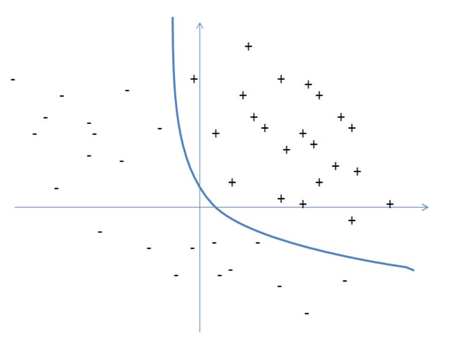

a , . . . , a and an intercept b, that separates the positive and negative points:
1
d0
0
Xd
i
a · ϕ(p ) + b > 0
(12)
(13)
j
j
i=1
for all positive points and
0
Xd
i
a · ϕ(q ) + b < 0
j
j
i=1
for all negative points. Note that if the new feature set includes all of the original features,
as in (10), then every hyperplane in the original d-dimensional space remains available in
the expanded space (just set ad+1, ad+2, . . . , ad0 = 0). But there are also many new options,
and hence it is more likely that there is way to perfectly separate the (images under ϕ of
the) data points. For example, even with d = 1 and the map (11), linear functions in the
expanded space have the form h(z) = a z2 + a z + b, which is a quadratic function in the
1
2
original space.
We can think of the map ϕ as being applied in a preprocessing step. Then, the resulting
problem of meeting all the constraints (12) and (13) is exactly the problem that we already
solved in Section 3.4. The resulting linear program has decision variables δ, a , . . . , a , b
1
d0
(d0 + 2 in all, up from d + 2 in the original space).16
1
6The magic of support vector machines is that, for many maps ϕ including (10) and (11), and for many
methods of computing a separating hyperplane, the computation required scales only with the original
dimension d, even if the expanded dimension d0 is radically larger. This is known as the “kernel trick;” see
CS229 for more details.
1
4

CS261: A Second Course in Algorithms
Lecture #8: Linear Programming Duality (Part 1)∗
Tim Roughgarden†
January 28, 2016
1
Warm-Up
This lecture begins our discussion of linear programming duality, which is the really the
heart and soul of CS261. It is the topic of this lecture, the next lecture, and (as will become
clear) pretty much all of the succeeding lectures as well.
Recall from last lecture the ingredients of a linear program: decision variables, linear
constraints (equalities or inequalities), and a linear objective function. Last lecture we saw
that lots of interesting problems in combinatorial optimization and machine learning reduce
to linear programming.
Figure 1: A toy example to illustrate duality.
∗
†
ꢀc
2
Department of Computer Science, Stanford University, 474 Gates Building, 353 Serra Mall, Stanford,
016, Tim Roughgarden.
CA 94305. Email: tim@cs.stanford.edu.
1
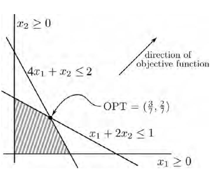

To start getting a feel for linear programming duality, let’s begin with a toy example. It
is a minor variation on our toy example from last time. There are two decision variables x1
and x2 and we want to
max x1 + x2
(1)
subject to
4
x + x ≤ 2
(2)
(3)
(4)
(5)
1
2
x + 2x ≤ 1
1
2
x ≥ 0
1
x ≥ 0.
2
(Last lecture, the first constraint of our toy example read 2x + x ≤ 1; everything else is
1
2
the same.)
Like last lecture, we can solve this LP just by eyeballing the feasible region (Figure 1)
and searching for the “most northeastern” feasible point, which in this case is the vertex
3
7
2
7
5
7
(i.e., “corner”) at ( , ). Thus the optimal objective function value if .
When we go beyond three dimensions (i.e., decision variables), it seems hopeless to solve
linear programs by inspection. With a general linear program, even if we are handed on a
silver platter an allegedly optimal solution, how do we know that it is really is optimal?
Let’s try to answer this question at least in our toy example. What’s an easy and
convincing proof that the optimal objective function value of the linear program can’t be
too large? For starters, for any feasible point (x , x ), we certainly have
1
2
x + x ≤ 4x + x ≤
objective
2
,
|
1 {z }2
1
2
|
{z}
upper bound
with the first inequality following from x ≥ 0 and the second from the first constraint. We
1
can immediately conclude that the optimal value of the linear program is at most 2. But
actually, it’s obvious that we can do better by using the second constraint instead:
x + x ≤ x + 2x ≤ 1,
1
2
1
2
giving us a better (i.e., smaller) upper bound of 1. Can we do better? There’s no reason
we need to stop at using just one constraint at a time, and are free to blend two or more
1
7
3
7
constraints. The best blending takes of the first constraint and of the second to give
1
7
3
7
5
x + x ≤ (4x + x ) + (x + 2x )
1
7
3
≤
·
2 +
·
1 = .
(6)
1
2
1
2
1
2
|
{z
}
7 | {z
}
7
≤
2 by (2)
≤ 1 by (3)
(The first inequality actually holds with equality, but we don’t need the stronger statement.)
5
So this is a convincing proof that the optimal objective function value is at most . Given
7
the feasible point ( , ) that actually does realize this upper bound, we can conclude that
3
2
5
7
7
really is the optimal value for the linear program.
7
2


Summarizing, for the linear program (1)–(5), there is a quick and convincing proof that
5
3
2
the optimal solution has value at least (namely, the feasible point ( , )) and also such a
5
7
proof that the optimal solution has value at most (given in (6)). This is the essence of
7
7
7
linear programming duality.
2
The Dual Linear Program
We now generalize the ideas of the previous section. Consider an arbitrary linear program
(call it (P)) of the form
Xn
max
cjxj
(7)
j=1
subject to
Xn
a x ≤ b
(8)
(9)
1
j
j
1
2
j=1
Xn
a x ≤ b
2
j
j
j=1
.
.
.
.
.
≤ .
(10)
(11)
Xn
a x ≤ b
mj
j
m
j=1
x , . . . , x ≥ 0.
(12)
1
n
This linear program has n nonnegative decision variables x , . . . , x and m constraints (not
1
counting the nonnegativity constraints). The a ’s, b ’s, and c ’s are all part of the input
n
ij
i
j
(i.e., fixed constants).1
You may have forgotten your linear algebra, but it’s worth paging the basics back in
when learning linear programming duality. It’s very convenient to write linear programs in
matrix-vector notation. For example, the linear program above translates to the succinct
description
max cT x
subject to
Ax ≤ b
x ≥ 0,
1
Remember that different types of linear programs are easily transformed to each other. A minimization
objective can be turned into a maximization objective by multiplying all cj’s by -1. An equality constraint
can be simulated by two inequality constraints. An inequality constraint can be flipped by multiplying by
-1. Real-valued decision variables can be simulated by the difference of two nonnegative decision variables.
An inequality constraint can be turned into an equality constraint by adding an extra “slack” variable.
3


where c and x are n-vectors, b is an m-vector, A is an m × n matrix (of the a ’s), and the
ij
inequalities are componentwise.
Remember our strategy for deriving upper bounds on the optimal objective function
value of our toy example: take a nonnegative linear combination of the constraints that
(componentwise) dominates the objective function. In general, for the above linear program
with m constraints, we denote by y , . . . , y ≥ 0 the corresponding multipliers that we use.
1
m
The goal of dominating the objective function translates to the conditions
Xm
y a ≥ c
(13)
i
ij
j
i=1
for each objective function coefficient (i.e. for j = 1, 2, . . . , m). In matrix notation, we are
interested in nonnegative m-vectors y ≥ 0 such that
AT y ≥ c;
note the sum in (13) is over the rows i of A, which corresponds to an inner product with the
jth column of A, or equivalently with the jth row of AT .
By design, every such choice of multipliers y1, . . . , ym implies an upper bound on the
optimal objective function value of the linear program (7)–(12): for every feasible solution
(x , . . . , x ),
1
n
!
Xn
x’s obj fn
Xn Xm
c x ≤
yiaij xj
(14)
j
j
j=1
j=1
i=1
|
{z }
!
Xm
Xn
=
yi ·
a xj
ij
(15)
(16)
i=1
j=1
Xm
upper bound
≤
y b . .
i i
i=1
|
{z }
In this derivation, inequality (14) follows from the domination condition in (13) and the
nonnegativity of x , . . . , x ; equation (15) follows from reversing the order of summation;
1
n
and inequality (16) follows from the feasibility of x and the nonnegativity of y , . . . , y .
1
Alternatively, the derivation may be more transparent in matrix-vector notation:
m
T
T
T
T
t
c x ≤ (A y) x = y (Ax) ≤ y b.
The upshot is that, whenever y ≥ 0 and (13) holds,
Xm
OPT of (P) ≤
b y .
i
i
i=1
4


In our toy example of Section 1, the first upper bound of 2 corresponds to taking y1 = 1
and y = 0. The second upper bound of 1 corresponds to y = 0 and y = 1 The final upper
2
1
2
5
7
1
7
3
7
bound of corresponds to y1 = and y = .
2
Our toy example illustrates that there can be many different ways of choosing the yi’s,
and different choices lead to different upper bounds on the optimal value of the linear pro-
gram (P). Obviously, the most interesting of these upper bounds is the tightest (i.e., smallest)
one. So we really want to range over all possible y’s and consider the minimum such upper
bound.2
Here’s the key point: the tightest upper bound on OPT is itself the optimal solution to a
linear program. Namely:
Xm
min
biyi
i=1
subject to
Xm
a y ≥ c
i1
i
1
2
i=1
Xm
a y ≥ c
i2
i
i=1
.
.
.
.
.
≥ .
Xm
a y ≥ c
in
i
n
i=1
y , . . . , y ≥ 0.
1
m
Or, in matrix-vector form:
subject to
min bT y
AT y ≥ c
y ≥ 0.
This linear program is called the dual to (P), and we sometimes denote it by (D).
For example, to derive the dual to our toy linear program, we just swap the objective
and the right-hand side and take the transpose of the constraint matrix:
min 2y1 + y2
2
For an analogy, among all s-t cuts, each of which upper bounds the value of a maximum flow, the
minimum cut is the most interesting one (Lecture #2). Similarly, in the Tutte-Berge formula (Lecture #5),
we were interested in the tightest (i.e., minimum) upper bound of the form |V | − (oc(S) − |S|), over all
choices of the set S.
5


subject to
4
y + y ≥ 1
1
2
y + 2y ≥ 1
1
2
y , y ≥ 0.
1
2
1
3
The objective function values of the feasible solutions (1, 0), (0, 1), and ( , ) (of 2, 1, and
7
7
5
7
)
correspond to our three upper bounds in Section 1.
The following important result follows from the definition of the dual and the deriva-
tion (14)–(16).
Theorem 2.1 (Weak Duality) For every linear program of the form (P) and correspond-
ing dual linear program (D),
OPT value for (P) ≤ OPT value for (D).
(17)
(Since the derivation (14)–(15) applies to any pair of feasible solutions, it holds in particular
for a pair of optimal solutions.) Next lecture we’ll discuss strong duality, which asserts
that (17) always holds with equality (as long as both (P) and (D) are feasible).
3
Duality Example #1: Max-Flow/Min-Cut Revisited
This section brings linear programming duality back down to earth by relating it to an old
friend, the maximum flow problem. Last lecture we showed how this problem translates easily
to a linear program. This lecture, for convenience, we will use a different linear programming
formulation. The new linear program is much bigger but also simpler, so it is easier to take
and interpret its dual.
3
.1 The Primal
The idea is to work directly with path decompositions, rather than flows. So the decision
variables have the form f , where P is an s-t path. Let P denote the set of all such paths.
P
The benefit of working with paths is that there is no need to explicitly state the conservation
constraints. We do still have the capacity (and nonnegativity) constraints, however.
X
max
fP
(18)
P∈P
subject to
X
fP ≤ ue
for all e ∈ E
(19)
(20)
P∈P : e∈P
|
{z
}
total flow on e
f ≥ 0
for all P ∈ P.
P
6


Again, call this (P). The optimal value to this linear program is the same as that of the linear
programming formulation of the maximum flow problem given last lecture. Every feasible
solution to (18)–(20) can be transformed into one of equal value for last lecture’s LP, just by
setting fe equal to the left-hand side of (19) for each e. For the reverse direction, one takes
a path decomposition (Problem Set #1). See Exercise Set #4 for details.
3
.2 The Dual
The linear program (18)–(20) conforms to the format covered in Section 2, so it has a well-
defined dual. What is it? It’s usually easier to take the dual in matrix-vector notation:
max 1T f
subject to
Af ≤ u
f ≥ 0,
where the vector f is indexed by the paths P, 1 stands for the (|P|-dimensional) all-ones
vector, u is indexed by E, and A is a P × E matrix. Then, the dual (D) has decision
variables indexed by E (denoted {` }
for reasons to become clear) and is
e
e∈E
min uT `
T
A ` ≥ 1
`
≥ 0.
Typically, the hardest thing about understanding a dual is interpreting what the transpose
operation on the constraint matrix (A → AT ) is doing. By definition, each row (correspond-
ing to an edge e) of A has a 1 in the column corresponding to a path P if e ∈ P, and 0
otherwise. So an entry aeP of A is 1 if e ∈ P and 0 otherwise. In the column of A (and hence
row of AT ) corresponding to a path P, there is a 1 in each row corresponding an edge e of P
(and zeroes in the other rows).
Now that we understand AT , we can unpack the dual and write it as
X
min
u `
e e
e∈E
subject to
X
`e ≥ 1
for all P ∈ P
for all e ∈ E.
(21)
e∈P
`e ≥ 0
7
3
.3 Interpretation of Dual
The duals of natural linear programs are often meaningful in their own right, and this one
is a good example. A key observation is that every s-t cut corresponds to a feasible solution
to this dual linear program. To see this, fix a cut (A, B), with s ∈ A and t ∈ B, and set
ꢀ
1
0
if e ∈ δ+(A)
`e
=
otherwise.
(Recall that δ+(A) denotes the edges sticking out of A, with tail in A and head in B; see
Figure 2.) To verify the constraints (21) and hence feasibility for the dual linear program,
note that every s-t path must cross the cut (A, B) as some point (since it starts in A and
ends in B). Thus every s-t path has at least one edge e with `e = 1, and (21) holds. The
objective function value of this feasible solution is
X
X
u ` =
e e
ue = capacity of (A, B),
e∈E
e∈δ+(A)
where the second equality is by definition (recall Lecture #2).
s-t-cuts correspond to one type of feasible solution to this dual linear program, where
every decision variable is set to either 0 or 1. Not all feasible solutions have this property:
any assignment of nonnegative “lengths” `e to the edges of G satisfying (21) is feasible. Note
that (21) is equivalent to the constraint that the shortest-path distance from s to t, with
respect to the edge lengths {`e}e∈E, is at least 1.3
Figure 2: δ+(A) denotes the two edges that point from A to B.
3
.4 Relation to Max-Flow/Min-Cut
Summarizing, we have shown that
max flow value = OPT of (P) ≤ OPT of (D) ≤ min cut value.
(22)
3
To give a simple example, in the graph s → v → t, one feasible solution assigns `sv = `vt = 12 . If the
edge (s, v) and (v, t) have the same capacity, then this is also an optimal solution.
8
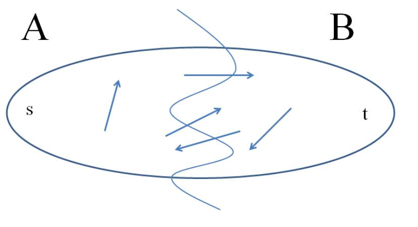


The first equation is just the statement the maximum flow problem can be formulated as
the linear program (P). The first inequality is weak duality. The second inequality holds
because the feasible region of (D) includes all (0-1 solutions corresponding to) s-t cuts; since
it minimizes over a superset of the s-t cuts, the optimal value can only be less than that of
the minimum cut.
In Lecture #2 we used the Ford-Fulkerson algorithm to prove the maximum flow/minimum
cut theorem, stating that there is never a gap between the maximum flow and minimum cut
values. So the first and last terms of (22) are equal, which means that both of the inequalities
are actually equalities. The fact that
OPT of (P) = OPT of (D)
is interesting because it proves a natural special case of strong duality, for flow linear pro-
grams and their duals. The fact that
OPT of (D) = min cut value
is interesting because it implies that the linear program (D), despite allowing fractional
solutions, always admits an optimal solution in which each decision variable is either 0 or 1.
3
.5 Take-Aways
The example in this section illustrates three general points.
1
2
. The duals of natural linear programs are often natural in their own right.
. Strong duality. ( We verified it in a special case, and will prove it in general next
lecture.)
3
. Some natural linear programs are guaranteed to have integral optimal solutions.
4
Recipe for Taking Duals
Section 2 defines the dual linear program for primal linear programs of a specific form
(maximization objective, inequality constraints, and nonnegative decision variables). As
we’ve mentioned, different types of linear programs are easily converted to each other. So
one perfectly legitimate way to take the dual of an arbitrary linear program is to first convert
it into the form in Section 2 and then apply that definition. But it’s more convenient to be
able to take the dual of any linear program directly, using a general recipe.
The high-level points of the recipe are familiar: dual variables correspond to primal
constraints, dual constraints correspond to primal variables, maximization and minimization
get exchanged, the objective function and right-hand side get exchanged, and the constraint
matrix gets transposed. The details concern the different type of constraints (inequality vs.
equality) and whether or not decision variables are nonnegative.
Here is the general recipe for maximization linear programs:
9
Primal
variables x1, . . . , xn
m constraints
objective function c
right-hand side b
max cT x
Dual
n constraints
variables y1, . . . , ym
right-hand side c
objective function b
min bT y
constraint matrix A constraint matrix AT
ith constraint is “≤”
ith constraint is “≥”
ith constraint is “=”
x ≥ 0
y ≥ 0
i
y ≤ 0
i
y ∈ R
i
jth constraint is “≥”
j
x ≤ 0
jth constraint is “≤”
jth constraint is “=”
j
x ∈ R
j
For minimization linear programs, we define the dual as the reverse operation (from the right
column to the left). Thus, by definition, the dual of the dual is the original primal.
5
Weak Duality
The above recipe allows you to take duals in a mechanical way, without thinking about
it. This can be very useful, but don’t forget the true meaning of the dual (which holds in
all cases): feasible dual solutions correspond to bounds on the best-possible primal objective
function value (derived from taking linear combinations of the constraints), and the optimal
dual solution is the tightest-possible such bound.
If you remember the meaning of duals, then it’s clear that weak duality holds in all cases
(essentially by definition).4
Theorem 5.1 (Weak Duality) For every maximization linear program (P) and corre-
sponding dual linear program (D),
OPT value for (P) ≤ OPT value for (D);
for every minimization linear program (P) and corresponding dual linear program (D),
OPT value for (P) ≥ OPT value for (D).
Weak duality can be visualized as in Figure 3. Strong duality also holds in all cases; see next
lecture.
4
Math classes often teach mathematical definitions as if they fell from the sky. This is not representative
of how mathematics actually develops. Typically, definitions are reverse engineered so that you get the
right” theorems (like weak/strong duality).
“
1
0


Figure 3: visualization of weak duality. X represents feasible solutions for P while O repre-
sents feasible solutions for D.
Weak duality already has some very interesting corollaries.
Corollary 5.2 Let (P),(D) be a primal-dual pair of linear programs.
(a) If the optimal objective function value of (P) is unbounded, then (D) is infeasible.
(b) If the optimal objective function value of (D) is unbounded, then (P) is infeasible.
(c) If x, y are feasible for (P),(D) and cT x = yT b, then both x and y are both optimal.
Parts (a) and (b) hold because any feasible solution to the dual of a linear program offers
a bound on the best-possible objective function value of the primal (so if there is no such
bound, then there is no such feasible solution). The hypothesis in (c) asserts that Figure 3
contains an “x” and an “o” that are superimposed. It is immediate that no other primal
solution can be better, and that no other dual solution can be better. (For an analogy, in
Lecture #2 we proved that capacity of every cut bounds from above the value of every flow,
so if you ever find a flow and a cut with equal value, both must be optimal.)
1
1

CS261: A Second Course in Algorithms
Lecture #9: Linear Programming Duality (Part 2)∗
Tim Roughgarden†
February 2, 2016
1
Recap
This is our third lecture on linear programming, and the second on linear programming
duality. Let’s page back in the relevant stuff from last lecture.
One type of linear program has the form
Xn
max
cjxj
j=1
subject to
Xn
a x ≤ b
1
j
j
1
2
j=1
Xn
a x ≤ b
2
j
j
j=1
.
.
.
.
.
≤ .
Xn
a x ≤ b
mj
j
m
j=1
x , . . . , x ≥ 0.
1
n
Call this linear program (P), for “primal.” Alternatively, in matrix-vector notation it is
max cT x
∗
†
ꢀc
2
Department of Computer Science, Stanford University, 474 Gates Building, 353 Serra Mall, Stanford,
016, Tim Roughgarden.
CA 94305. Email: tim@cs.stanford.edu.
1

subject to
Ax ≤ b
x ≥ 0,
where c and x are n-vectors, b is an m-vector, A is an m × n matrix (of the a ’s), and the
ij
inequalities are componentwise.
We then discussed a method for generating upper bounds on the maximum-possible
objective function value of (P): take a nonnegative linear combination of the constraints
so that the result dominates the objective c, and you get an upper bound equal to the
corresponding nonnegative linear combination of the right-hand side b. A key point is that
the tightest upper bound of this form is the solution to another linear program, known as
the “dual.” We gave a general recipe for taking duals: the dual has one variable per primal
constraint and one constraint per primal variable; “max” and “min” get interchanged; the
objective function and the right-hand side get interchanged; and the constraint matrix gets
transposed. (There are some details about whether decision variables are nonnegative or
not, and whether the constraints are equalities or inequalities; see the table last lecture.)
For example, the dual linear program for (P), call it (D), is
min yT b
subject to
T
A y ≥ c
y ≥ 0
in matrix-vector form. Or, if you prefer the expanded version,
Xm
min
biyi
i=1
subject to
Xm
a y ≥ c
i1
i
1
2
i=1
Xm
a y ≥ c
i2
i
i=1
.
.
.
.
.
≥ .
Xm
a y ≥ c
in
i
n
i=1
y , . . . , y ≥ 0.
1
m
2
In all cases, the meaning of the dual is the tightest upper bound that can proved on
the optimal primal objective function by taking suitable linear combinations of the primal
constraints. With this understanding, we see that weak duality holds (for all forms of LPs),
essentially by construction.
For example, for a primal-dual pair (P),(D) of the form above, for every pair x, y of
feasible solutions to (P),(D), we have
!
Xn
x’s obj fn
Xn Xm
c x ≤
yiaij xj
(1)
j
j
j=1
j=1
i=1
|
{z }
!
Xm
Xn
=
yi
a xj
ij
(2)
(3)
i=1
j=1
Xm
y’s obj fn
≤
y b .
i i
i=1
|
{z }
Or, in matrix-vector notion,
T
T
T
T
t
c x ≤ (A y) x = y (Ax) ≤ y b.
The first inequality uses that x ≥ 0 and Aty ≥ c; the second that y ≥ 0 and Ax ≤ b.
We concluded last lecture with the following sufficient condition for optimality.1
Corollary 1.1 Let (P),(D) be a primal-dual pair of linear programs. If x, y are feasible
solutions to (P),(D), and cT x = yT b, then both x and y are both optimal.
For the reason, recall Figure 1 — no “x” can be to the right of an “o”, so if an “x” and
“o” are superimposed it must be the rightmost “x” and the leftmost “o.” For an analogy,
whenever you find a flow and s-t cut with the same value, the flow must be maximum and
the cut minimum.
Figure 1: Illustrative figure showing feasible solutions for the primal (x) and the dual (o).
1
We also noted that weak duality implies that whenever the optimal objective function of (P) is unbounded
the linear program (D) is infeasible, and vice versa.
3


2
Complementary Slackness Conditions
2
.1 The Conditions
Next is a corollary of Corollary 1.1. It is another sufficient (and as we’ll see later, necessary)
condition for optimality.
Corollary 2.1 (Complementary Slackness Conditions) Let (P),(D) be a primal-dual
pair of linear programs. If x, y are feasible solutions to (P),(D), and the following two
conditions hold then both x and y are both optimal.
(1) Whenever xj = 0, y satisfies the jth constraint of (D) with equality.
(2) Whenever yi = 0, x satisfies the ith constraint of (P) with equality.
The conditions assert that no decision variable and corresponding constraint are simultane-
ously “slack” (i.e., it forbids that the decision variable is not 0 and also the constraint is not
tight).
Proof of Corollary 2.1: We prove the corollary for the case of primal and dual programs of
the form (P) and (D) in Section 1; the other cases are all the same.
The first condition implies that
!
Xm
c x =
j
yiaij xj
j
i=1
P
m
i=1
for each j = 1, . . . , n (either x = 0 or c =
j
y a ). Hence, inequality (1) holds with
i ij
j
equality. Similarly, the second condition implies that
!
Xn
yi
a xi = y b
ij
i i
j=1
for each i = 1, . . . , m. Hence inequality (3) also holds with equality. Thus cT x = yT b, and
Corollary 1.1 implies that both x and y are optimal. ꢀ
4
2
.2 Physical Interpretation
Figure 2: Physical interpretation of complementary slackness. The objective function pushes
a particle in the direction c until it rests at x∗. Walls also exert a force on the particle, and
complementary slackness asserts that only walls touching the particle exert a force, and sum
of forces is equal to 0.
We offer the following informal physical metaphor for the complementary slackness condi-
tions, which some students find helpful (Figure 2). For a linear program of the form (P) in
Section 1, think of the objective function as exerting “force” in the direction c. This pushes
a particle in the direction c (within the feasible region) until it cannot move any further in
this direction. When the particle comes to rest at position x∗, the sum of the forces acting on
it must sum to 0. What else exerts force on the particle? The “walls” of the feasible region,
corresponding to the constraints. The direction of the force exerted by the ith constraint of
P
n
j=1
the form
the constraint matrix. We can interpret the corresponding dual variable y as the magnitude
a x ≤ b is perpendicular to the wall, that is, −a , where a is the ith row of
ij
j
i
i
i
i
of the force exerted in this direction −a . The assertion that the sum of the forces equals 0
P
i
y a . The complementary slackness conditions assert
n
i=1
corresponds to the equation c =
i
i
that y > 0 only when aT x = b — that is, only the walls that the particle touches are
i
allowed to exert force on it.
i
i
2
.3 A General Algorithm Design Paradigm
So why are the complementary slackness conditions interesting? One reason is that they
offer three principled strategies for designing algorithms for solving linear programs and
their special cases. Consider the following three conditions.
A General Algorithm Design Paradigm
1
. x is feasible for (P).
5
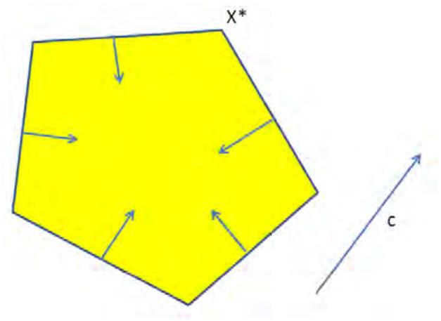

2
3
. y is feasible for (D).
. x, y satisfy the complementary slackness conditions (Corollary 2.1).
Pick two of these three conditions to maintain at all times, and work
toward achieving the third.
By Corollary 2.1, we know that achieving these three conditions simultaneously implies that
both x and y are optimal. Each choice of a condition to relax offers a disciplined way
of working toward optimality, and in many cases all three approaches can lead to good
algorithms. Countless algorithms for linear programs and their special cases can be viewed
as instantiations of this general paradigm. We next revisit an old friend, the Hungarian
algorithm, which is a particularly transparent example of this design paradigm in action.
3
Example #2: The Hungarian Algorithm Revisited
3
.1 Recap of Example #1
Recall that in Lecture #8 we reinterpreted the max-flow/min-cut theorem through the lens
of LP duality (this was “Example #1”). We had a primal linear program formulation of
the maximum flow problem. In the corresponding dual linear program, we observed that s-t
cuts translate to 0-1 solutions to this dual, with the dual objective function value equal to
the capacity of the cut. Using the max-flow/min-cut theorem, we concluded two interesting
properties: first, we verified strong duality (i.e., no gap between the optimal primal and dual
objective function values) for primal-dual pairs corresponding to flows and (fractional) cuts;
second, we concluded that these dual linear programs are always guaranteed to possess an
integral optimal solution (i.e., fractions don’t help).
3
.2 The Primal Linear Program
Back in Lecture #7 we claimed that all of the problems studied thus far are special cases
of linear programs. For the maximum flow problem, this is easy to believe, because flows
can be fractional. But for matchings? They are suppose to be integral, so how could they
be modeled with a linear program? Example #1 provides the clue — sometimes, linear
programs are guaranteed to have an optimal integral solution. As we’ll see, this also turns
out to be the case for bipartite matching.
Given a bipartite graph G = (V ∪ W, E) with a cost ce for each edge, the relevant linear
program (P-BM) is
X
min
cexe
e∈E
6

subject to
X
xe = 1
xe ≥ 0
for all v ∈ V ∪ W
for all e ∈ E,
e∈δ(v)
where δ(v) denotes the edges incident to v. The intended semantics is that each xe is either
equal to 1 (if e is in the chosen matching) or 0 (otherwise). Of course, the linear program is
also free to use fractional values for the decision variables.2
In matrix-vector form, this linear program is
min cT x
subject to
Ax = 1
x ≥ 0,
where A is the (V ∪ W) × E matrix
ꢀ
ꢁ
ꢂ
1
0
if e ∈ δ(v)
A = a =
ve
(4)
otherwise
3
.3 The Dual Linear Program
We now turn to the dual linear program. Note that (P-BM) differs from our usual form
both by having a minimization objective and by having equality (rather than inequality)
constraints. But our recipe for taking duals from Lecture #8 applies to all types of linear
programs, including this one.
When taking a dual, usually the trickiest point is to understand the effect of the transpose
operation (on the constraint matrix). In the constraint matrix A in (4), each row (indexed
by v ∈ V ∪ W) has a 1 in each column (indexed by e ∈ E) for which e is incident to v (and
0
s in other columns). Thus, a column of A (and hence row of AT ) corresponding to edge e
has 1s in precisely the rows (indexed by v) such that e is incident to v — that is, in the two
rows corresponding to e’s endpoints.
Applying our recipe for duals to (P-BM), initially in matrix-vector form for simplicity,
yields
max pT 1
subject to
T
A p ≤ c
p ∈ R .
E
2
If you’re tempted to also add in the constraints that x ≤ 1 for every e ∈ E, note that these are already
e
implied by the current constraints (why?).
7

We are using the notation p for the dual variable corresponding to a vertex v ∈ V ∪ W, for
v
reasons that will become clearly shortly. Note that these decision variables can be positive
or negative, because of the equality constraints in (P-BM).
Unpacking this dual linear program, (D-BM), we get
X
max
pv
v∈V ∪W
subject to
p + p ≤ c
for all (v, w) ∈ E
for all v ∈ V ∪ W.
v
w
vw
p ∈ R
v
Here’s the punchline: the “vertex prices” in the Hungarian algorithm (Lecture #5) corre-
spond exactly to the decision variables of the dual (D-BM). Indeed, without thinking about
this dual linear program, how would you ever think to maintain numbers attached to the
vertices of a graph matching instance, when the problem definition seems to only concern
the graph’s edges?3
It gets better: rewrite the constraints of (D-BM) as
c
− p − p ≥ 0
reduced cost
(5)
vw
v
w
|
{z
}
for every edge (v, w) ∈ E. The left-hand side of (5) is exactly our definition in the Hungarian
algorithm of the “reduced cost” of an edge (with respect to prices p). Thus the first invariant
of the Hungarian algorithm, asserting that all edges have nonnegative reduced costs, is
exactly the same as maintaining the dual feasibility of p!
To seal the deal, let’s check out the complementary slackness conditions for the primal-
dual pair (P-BM),(D-BM). Because all constraints in (P-BM) are equations (not counting
the nonnegativity constraints), the second condition is trivial. The first condition states
that whenever xe > 0, the corresponding constraint (5) should hold with equality — that is,
edge e should have zero reduced cost. Thus the second invariant of the Hungarian algorithm
(that edges in the current matching should be “tight”) is just the complementary slackness
condition!
We conclude that, in terms of the general algorithm design paradigm in Section 2.3,
the Hungarian algorithm maintains the second two conditions (p is feasible for (D-BM)
and complementary slackness conditions) at all times, and works toward the first condition
(primal feasibility, i.e., a perfect matching). Algorithms of this type are called primal-dual
algorithms, and the Hungarian algorithm is a canonical example.
3
In Lecture #5 we motivated vertex prices via an analogy with the vertex labels maintained by the push-
relabel maximum flow algorithm. But the latter is from the 1980s and the former from the 1950s, so that
was a pretty ahistorical analogy. Linear programming (and duality) were only developed in the late 1940s,
and so it was a new subject when Kuhn designed the Hungarian algorithm. But he was one of the first
masters of the subject, and he put his expertise to good use.
8


3
.4 Consequences
We know that
OPT of (D-PM) ≤ OPT of (P-PM) ≤ min-cost perfect matching.
(6)
The first inequality is just weak duality (for the case where the primal linear program has
a minimization objective). The second inequality follows from the fact that every perfect
matching corresponds to a feasible (0-1) solution of (P-BM); since the linear program min-
imizes over a superset of these solutions, it can only have a better (i.e., smaller) optimal
objective function value.
In Lecture #5 we proved that the Hungarian algorithm always terminates with a perfect
matching (provided there is at least one). The algorithm maintains a feasible dual and the
complementary slackness conditions. As in the proof of Corollary 2.1, this implies that the
cost of the constructed perfect matching equals the dual objective function value attained
by the final prices. That is, both inequalities in (6) must hold with equality.
As in Example #1 (max flow/min cut), both of these equalities are interesting. The first
equation verifies another special case of strong LP duality, for linear programs of the form
(P-BM) and (D-BM). The second equation provides another example of a natural family of
linear programs — those of the form (P-BM) — that are guaranteed to have 0-1 optimal
solutions.4
4
Strong LP Duality
4
.1 Formal Statement
Strong linear programming duality (“no gap”) holds in general, not just for the special cases
that we’ve seen thus far.
Theorem 4.1 (Strong LP Duality) When a primal-dual pair (P),(D) of linear programs
are both feasible,
OPT for (P) = OPT for (D).
Amazingly, our simple method of deriving bounds on the optimal objective function value of
(P) through suitable linear combinations of the constraints is always guaranteed to produce
the tightest-possible bound! Strong duality can be thought of as a generalization of the max-
flow/min-cut theorem (Lecture #2) and Hall’s theorem (Lecture #5), and as the ultimate
answer to the question “how do we know when we’re done?”5
4
5
See also Exercise Set #4 for a direct proof of this.
When at least one of (P),(D) is infeasible, there are three possibilities, all of which can occur. First, (P)
might have unbounded objective function value, in which case (by weak duality) (D) is infeasible. It is also
possible that (P) is infeasible while (D) has unbounded objective function value. Finally, sometimes both
(P) and (D) are infeasible (an uninteresting case).
9

4
.2 Consequent Optimality Conditions
Strong duality immediately implies that the sufficient conditions for optimality identified
earlier (Corollaries 1.1 and 2.1) are also necessary conditions — that is, they are optimality
conditions in the sense derived earlier for the maximum flow and minimum-cost perfect
bipartite matching problems.
Corollary 4.2 (LP Optimality Conditions) Let x, y are feasible solutions to the primal-
dual pair (P),(D) be a = primal-dual pair, then
T
x, y are both optimal if and only if c x = y b
T
if and only if the complementary slackness conditions hold.
The first if and only if follows from strong duality: since both (P),(D) are feasible by as-
∗ T
∗
∗
∗
sumption, strong duality assures us of feasible solutions x , y with cx = (y ) b. If x, y
fail to satisfy this equality, then either cT x is worse than cT x or y b is worse than (y ) b
(or both). The second if and only if does not require strong duality; it follows from the proof
of Corollary 2.1 (see also Exercise Set #4).
∗
T
∗ T
4
.3 Proof Sketch: The Road Map
We conclude the lecture with a proof sketch of Theorem 4.1. Our proof sketch leaves some
details to Problem Set #3, and also takes on faith one intuitive geometric fact. The goal of
the proof sketch is to at least partially demystify strong LP duality, and convince you that
it ultimately boils down to some simple geometric intuition.
Here’s the plan:
separating hyperplane ⇒ Farkas’s Lemma → strong LP duality .
|
{z
}
|
{z
}
|
{z
}
will prove
will assume
PSet #3
The “separating hyperplane theorem” is the intuitive geometric fact that we assume (Sec-
tion 4.4). Section 4.5 derives from this fact Farkas’s Lemma, a “feasibility version” of strong
LP duality. Problem Set #3 asks you to reduce strong LP duality to Farkas’s Lemma.
4
.4 The Separating Hyperplane Theorem
In Lecture #7 we discussed separating hyperplanes, in the context of separating data points
labeled “positive” from those labeled “negative.” There, the point was to show that the
computational problem of finding such a hyperplane reduces to linear programming. Here,
we again discuss separating hyperplanes, with two differences: first, our goal is to separate
a convex set from a point not in the set (rather than two different sets of points); second,
the point here is to prove strong LP duality, not to give an algorithm for a computational
problem.
We assume the following result.
1
0


Theorem 4.3 (Separating Hyperplane) Let C be a closed and convex subset of Rn, and
z a point in Rn not in C. Then there is a separating hyperplane, meaning coefficients α ∈ Rn
and an intercept β ∈ R such that:
(1)
T
α x ≥ β
all of C on one side of hyperplane
for all x ∈ C;
|
{z
}
(2)
T
α z < β .
|
See also Figure 3. Note that the set C is not assumed to be bounded.
{z }
z on other side
Figure 3: Illustration of separating hyperplane theorem.
If you’ve forgotten what “convex” or “closed” means, both are very intuitive. A convex
set is “filled in,” meaning it contains all of its chords. Formally, this translates to
λx + (1 − λ)y
point on chord between x, y
∈ C
|
{z
}
for all x, y ∈ C and λ ∈ [0, 1]. See Figure 4 for an example (a filled-in polygon) and a
non-example (an annulus).
A closed set is one that includes its boundary.6 See Figure 5 for an example (the unit
disc) and a non-example (the open unit disc).
6
One formal definition is that whenever a sequence of points in C converges to a point x∗, then x∗ should
also be in C.
1
1


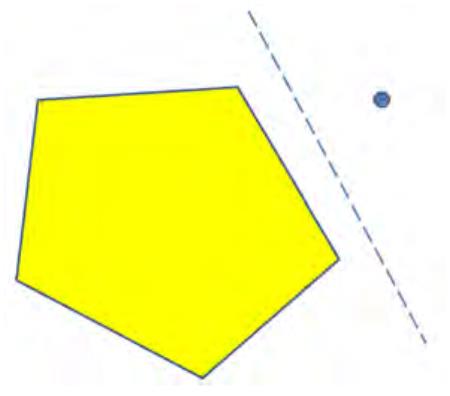


Figure 4: (a) a convex set (filled-in polygon) and (b) a non-convex set (annulus)
Figure 5: (a) a closed set (unit disc) and (b) non-closed set (open unit disc)
Hopefully Theorem 4.3 seems geometrically obvious, at least in two and three dimensions.
It turns out that the math one would use to prove this formally extends without trouble to
an arbitrary number of dimensions.7 It also turns out that strong LP duality boils down to
exactly this fact.
4
.5 Farkas’s Lemma
It’s easy to convince someone whether or not a system of linear equations has a solution: just
run Gaussian elimination and see whether or not it finds a solution (if there is a solution,
Gaussian elimination will find one). For a system of linear inequalities, it’s easy to convince
someone that there is a solution — just exhibit it and let them verify all the constraints. But
how would you convince someone that a system of linear inequalities has no solution? You
can’t very well enumerate the infinite number of possibilities and check that each doesn’t
work. Farkas’s Lemma is a satisfying answer to this question, and can be thought of as the
“
feasibility version” of strong LP duality.
Theorem 4.4 (Farkas’s Lemma) Given a matrix A ∈ Rm and a right-hand side b
×
n
∈
Rm, exactly one of the following holds:
(i) There exists x ∈ Rn such that x ≥ 0 and Ax = b;
(ii) There exists y ∈ Rm such that yT A ≥ 0 and yT b < 0.
7
If you know undergraduate analysis, then even the formal proof is not hard: let y be the nearest neighbor
to z in C (such a point exists because C is closed), and take a hyperplane perpendicular to the line segment
between y and z, through the midpoint of this segment (cf., Figure 3). All of C lies on the same side of this
hyperplane (opposite of z) because C is convex and y is the nearest neighbor of z in C.
1
2

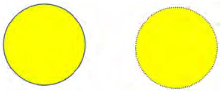

To connect the statement to the previous paragraph, think of Ax = b and x ≥ 0 as the
linear system of inequalities that we care about, and solutions to (ii) as proofs that this
system has no feasible solution.
Just like there are many variants of linear programs, there are many variants of Farkas’s
Lemma. Given Theorem 4.4, it is not hard to translate it to analogous statements for other
linear systems of inequalities (e.g., with both inequality and nonnegativity constraints); see
Problem Set #3.
Proof of Theorem 4.4: First, we have deliberately set up (i) and (ii) so that it’s impossible
for both to have a feasible solution. For if there were such an x and y, we would have
T
(y A) x ≥ 0
|
{z}
|
{z }
≥
0
≥
0
and yet
T
y (Ax) = y b < 0,
T
a contradiction. In this sense, solutions to (ii) are proofs of infeasibility of the the system (i)
(and vice versa).
But why can’t both (i) and (ii) be infeasible? We’ll show that this can’t happen by proving
that, whenever (i) is infeasible, (ii) is feasible. Thus the “proofs of infeasibility” encoded
by (ii) are all that we’ll ever need — whenever the linear system (i) is infeasible, there is
a proof of it of the prescribed type. There is a clear analogy between this interpretation
of Farkas’s Lemma and strong LP duality, which says that there is always a feasible dual
solution proving the tightest-possible bound on the optimal objective function value of the
primal.
Assume that (i) is infeasible. We need to somehow exhibit a solution to (ii), but where
could it come from? The trick is to get it from the separating hyperplane theorem (Theo-
rem 4.3) — the coefficients defining the hyperplane will turn out to be a solution to (ii). To
apply this theorem, we need a closed convex set and a point not in the set.
Define
Q = {d : ∃x ≥ 0 s.t. Ax = d}.
Note that Q is a subset of Rm. There are two different and equally useful ways to think
about Q. First, for the given constraint matrix A, Q is the set of all right-hand sides d
that are feasible (in x ≥ 0) with this constraint matrix. Thus by assumption, b ∈/ Q.
Equivalently, considering all vectors of the form Ax, with x ranging over all nonnegative
vectors in Rn, generates precisely the set of feasible right-hand sides. Thus Q equals the
set of all nonnegative linear combinations of the columns of A.8 This definition makes it
obvious that Q is convex (an average of two nonnegative linear combinations is just another
nonnegative linear combination). Q is also closed (the limit of a convergent sequence of
nonnegative linear combinations is just another nonnegative linear combination).
8
Called the “cone generated by” the columns of A.
1
3


Since Q is closed and convex and b ∈/ Q, we can apply Theorem 4.3. In return, we are
granted a coefficient vector α ∈ Rm and an intercept β ∈ R such that
αT d ≥ β
for all d ∈ Q and
αT b < β.
An exercise shows that, since Q is a cone, we can take β = 0 without loss of generality (see
Exercise Set #5). Thus
αT d ≥ 0
αT b < 0.
(7)
for all d ∈ Q while
(8)
A solution y to (ii) satisfies yT A ≥ 0 and yT b < 0. Suppose we just take y = α. Inequal-
ity (8) implies the second condition, so we just have to check that αT A ≥ 0. But what is
αT A? An n-vector, where the jth coordinate is inner product of αT and the jth column
aj of A. Since each aj ∈ Q — the jth column is obviously one particular nonnegative lin-
ear combination of A’s columns — inequality (7) implies that every coordinate of αT A is
nonnegative. Thus α is a solution to (ii), as desired. ꢀ
4
.6 Epilogue
On Problem Set #3 you will use Theorem 4.4 to prove strong LP duality. The idea is
simple: let OP T(D) denote the optimal value of the dual linear program, add a constraint to
the primal stating that the (primal) objective function value must be equal to or better than
OP T(D), and use Farkas’s Lemma to prove that this augmented linear program is feasible.
In summary, strong LP duality is amazing and powerful, yet it ultimately boils down to
the highly intuitive existence of a separating hyperplane between a closed convex set and a
point not in the set.
1
4
CS261: A Second Course in Algorithms
Lecture #10: The Minimax Theorem and Algorithms
for Linear Programming∗
Tim Roughgarden†
February 4, 2016
1
Zero-Sum Games and the Minimax Theorem
1
.1 Rock-Paper Scissors
Recall rock-paper-scissors (or roshambo). Two players simultaneously choose one of rock,
paper, or scissors, with rock beating scissors, scissors beating paper, and paper beating rock.1
Here’s an idea: what if I made you go first? That’s obviously unfair — whatever you do,
I can respond with the winning move.
But what if I only forced you to commit to a probability distribution over rock, paper,
and scissors? (Then I respond, then nature flips coins on your behalf.) If you prefer, imagine
that you submit your code for a (randomized) algorithm for choosing an action, then I have
to choose my action, and then we run your algorithm and see what happens.
In the second case, going first no longer seems to doom you. You can protect yourself by
randomizing uniformly among the three options — then, no matter what I do, I’m equally
likely to win, lose, or tie. The minimax theorem states that, in general games of “pure
competition,” a player moving first can always protect herself by randomizing appropriately.
∗
†
ꢀc
2
Department of Computer Science, Stanford University, 474 Gates Building, 353 Serra Mall, Stanford,
016, Tim Roughgarden.
CA 94305. Email: tim@cs.stanford.edu.
Here are some fun facts about rock-paper-scissors. There’s a World Series of RPS every year, with a top
1
prize of at least $50K. If you watch some videos of them, you will see pure psychological welfare. Maybe this
explains why some of the same players seem to end up in the later rounds of the tournament every year.
There’s also a robot hand, built at the University of Tokyo, that plays rock-paper-scissors with a winning
probability of 100% (check out the video). No surprise, a very high-speed camera is involved.
1

1
.2 Zero-Sum Games
A zero-sum game is specified by a real-valued matrix m × n matrix A. One player, the row
player, picks a row. The other (column) player picks a column. Rows and columns are also
called strategies. By definition, the entry aij of the matrix A is the row player’s payoff when
she chooses row i and the column player chooses column j. The column player’s payoff in
this case is defined as −a ; hence the term “zero-sum.” In effect, a is the amount that
ij
ij
the column player pays to the row player in the outcome (i, j). (Don’t forget, a might be
ij
negative, corresponding to a payment in the opposite direction.) Thus, the row and column
players prefer bigger and smaller numbers, respectively.
The following matrix describes the payoffs in the Rock-Paper-Scissors game in our current
language.
Rock Paper Scissors
Rock
Paper
Scissors
0
1
-1
-1
0
1
1
-1
0
1
.3 The Minimax Theorem
We can write the expected payoff of the row player when payoffs are given by an m × n
matrix A, the row strategy is x (a distribution over rows), and the column strategy is y (a
distribution over columns), as
Xm Xn
Xm Xn
Pr[outcome (i, j)] aij =
Pr[row i chosen] · Pr[column j chosen] a
ij
|
{z
} |
{z
}
i=1 j=1
i=1 j=1
=
x
=y
i
j
=
x>Ay.
The first term is just the definition of expectation, and the first equality holds because the
row and column players randomize independently. That is, x>Ay is just the expected payoff
to the row player (and negative payoff to the second player) when the row and column
strategies are x and y.
In a two-player zero-sum game, would you prefer to commit to a mixed strategy before or
after the other player commits to hers? Intuitively, there is only a first-mover disadvantage,
since the second player can adapt to the first player’s strategy. The minimax theorem is the
amazing statement that it doesn’t matter.
Theorem 1.1 (Minimax Theorem) For every two-player zero-sum game A,
ꢁ
ꢀ
ꢂ
On the left-hand side of (1), the row player moves first and the column player second. The
ꢃ
>
max min x Ay = min max x Ay .
>
(1)
x
y
y
x
column player plays optimally given the strategy chosen by the row player, and the row
2


player plays optimally anticipating the column player’s response. On the right-hand side
of (1), the roles of the two players are reversed. The minimax theorem asserts that, under
optimal play, the expected payoff of each player is the same in the two scenarios.
For example, in Rock-Paper-Scissors, both sides of (1) are 0 (with the first player playing
uniformly and the second player responding arbitrarily). When a zero-sum game is asym-
metric and skewed toward one of the players, both sides of (1) will be non-zero (but still
equal). The common number on both sides of (1) is called the value of the game.
1
.4 From LP Duality to Minimax
Theorem 1.1 was originally proved by John von Neumann in the 1920s, using fixed-point-
style arguments. Much later, in the 1940s, von Neumann proved it again using arguments
equivalent to strong LP duality (as we’ll do here). This second proof is the reason that,
when a very nervous George Dantzig (more on him later) explained his new ideas about
linear programming and the simplex method to von Neumann, the latter was able, off the
top of his head, to immediately give an hour-plus response that outlined the theory of LP
duality.
We now proceed to derive Theorem 1.1 from LP duality. The first step is to formalize
the problem of computing the best strategy for the player forced to go first.
Looking at the left-hand side (say) of (1), it doesn’t seem like linear programming should
apply. The first issue is the nested min/max, which is not allowed in a linear program. The
second issue is the quadratic (nonlinear) character of x>Ay in the decision variables x, y.
But we can work these issues out.
A simple but important observation is: the second player never needs to randomize. For
example, suppose the row player goes first and chooses a distribution x. The column player
can then simply compute the expected payoff of each column (the expectation with respect
to x) and choose the best column (deterministically). If multiple columns are tied for the
best, the it is also optimal to randomized arbitrarily among these; but there is no need for
the player moving second to do so.
In math, we have argued that
ꢀ
ꢁ
ꢀ
ꢁ
n
max min x Ay = max min x Ae
T
T
j
x
y
x
j=1
!
Xm
n
max min
=
a xi
,
(2)
ij
x
j=1
i=1
where ej is the jth standard basis vector, corresponding to the column player deterministi-
cally choosing column j.
We’ve solved one of our problems by getting rid of y. But there is still the nested
max/min. Here we recall a trick from Lecture #7, that a minimum or maximum can often
be simulated by additional variables and constraints. The same trick works here, in exactly
the same way.
3
Specifically, we introduce a decision variable v, intended to be equal to (2), and
max v
subject to
Xm
v −
a x ≤ 0
for all j = 1, . . . , n
(3)
ij
i
i=1
Xm
xi = 1
i=1
x , . . . , x ≥ 0 and v ∈ R.
1
m
Note that this is a linear program. Rewriting the constraints (3) in the form
Xm
v ≤
a xi
ij
for all j = 1, . . . , n
i=1
P
makes it clear that they force v to be at most minn
m
a x .
j=1
i=1 ij
∗
i
We claim that if (v , x ) is an optimal solution, then v = min
P
∗
∗
n
j=1
m
a xi. This follows
i=1 ij
∗
from the same arguments used in Lecture #7. As already noted, by feasibility, v cannot
m
P
be larger than minn
a x . If it were strictly less, then we can increase v slightly
∗
∗
j=1
i=1 ij
i
without destroying feasibility, yielding a better feasible solution (contradicting optimality).
Since the linear program explicitly maximizes v over all distributions x, its optimal
objective function value is
ꢀ
ꢁ
ꢀ
ꢁ
n
v = max min x Ae = max min x Ay .
∗
>
>
(4)
j
x
j=1
x
y
Thus we can compute with a linear program the optimal strategy for the row player, when it
moves first, and the expected payoff obtained (assuming optimal play by the column player).
Repeating the exercise for the column player gives the linear program
min w
subject to
Xn
w −
a y ≥ 0
for all i = 1, . . . , m
ij
j
j=1
Xn
yj = 1
j=1
y , . . . , y ≥ 0 and w ∈ R.
1
n
4
∗
∗
∗
At an optimal solution (w , y ), y is the optimal strategy for the column player (when going
first, assuming optimal play by the row player) and
ꢂ
ꢃ
ꢂ
ꢃ
m
∗
w = min max e Ay = min max x Ay .
>
>
(5)
i
y
i=1
y
x
Here’s the punch line: these two linear programs are duals. This can be seen by looking
up our recipe for taking duals (Lecture #8) and verifying that these two linear programs
conform to the recipe (see Exercise Set #5). For example, the one unrestricted variable (v
P
n
j=1
or w) corresponds to the one equality constraint in the other linear program (
yj = 1
P
m
i=1
or
xi = 1, respectively).
∗
∗
Strong duality implies that v = w ; in light of (4) and (5), the minimax theorem follows
directly.2
2
Survey of Linear Programming Algorithms
We’ve established that linear programs capture lots of different problems that we’d like to
solve. So how do we efficiently solve a linear program?
2
.1 The High-Order Bit
If you only remember one thing about linear programming, make it this:
Linear programs can be solved efficiently, in both theory and practice.
By “in theory,” we mean that linear programs can be solved in polynomial time in the worst-
case. By “in practice,” we mean that commercial solvers routinely solve linear programs
with input size in the millions. (Warning: the algorithms used in these two cases are not
necessarily the same.)
2
.2 The Simplex Method
2
.2.1 Backstory
In 1947 George Dantzig developed both the general formalism of linear programming and
also the first general algorithm for solving linear programs, the simplex method.3 Amazingly,
the simplex method remains the dominant paradigm today for solving linear programs.
2
The minimax theorem is obviously interesting its own right, and it also has applications in algorithms,
specifically to proving lower bounds on what randomized algorithms can do.
Dantzig spent the final 40 years of his career at Stanford (1966-2005). You’ve probably heard the story
3
about a student who is late to class, sees two problems written on the blackboard, assumes they’re homework
problems, and then goes home and solves them, not realizing that they are the major open questions in the
field. (A partial inspiration for Good Will Hunting, among other things.) Turns out this story is not
apocryphal: it was Dantzig, as a PhD student in the late 1930s, in a statistics course at UC Berkeley.
5


2
.2.2 Geometry
Figure 1: Illustration of a feasible set and an optimal solution x∗. We know that there always
exists an optimal solution at a vertex of the feasible set, in the direction of the objective
function.
In Lecture #7 we developed geometric intuition about what it means to solve a linear
program, and one of our findings was that there is always an optimal solution at a vertex
(i.e., “corner”) of the feasible region (e.g., Figure 1).4 This observation implies a finite
(but bad) algorithm for linear programming. (This is not trivial, since there are an infinite
number of feasible solutions.) The reason is that every vertex satisfies at least n constraints
with equality (where n is the number of decision variables). Or contrapositively: for a
feasible solution x that satisfies at most n − 1 constraints with equality, there is a direction
along which moving x continues to satisfy these constraints, and moving x locally in either
direction on this line yields two feasible points whose midpoint is x. But a vertex of a feasible
region cannot be written as a non-trivial convex combination of other feasible points.5 See
also Exercise Set #5. The finite algorithm is then: enumerate all (finitely many) subsets of
n linearly independent constraints, check if the unique point of Rn that satisfies all of them
is a feasible solution to the linear program, and remember the best feasible solution found
in this way.
The simplex algorithm also searches through the vertices of the feasible region, but does
so in a smarter and more principled way. The basic idea is to use local search — if there is
a “neighboring” vertex which is better, move to it, otherwise halt. The idea of neighboring
vertices should be clear from Figure 1 — two endpoints of an “edge” of the feasible region.
In general, we can define two different vertices to be neighboring if and only if they satisfy
n − 1 common constraints with equality. Moving from one vertex to a neighbor then just
involves swapping out one of the old tight constraints for a new tight constraint; each such
swap (also called a pivot) corresponds to a “move” along an edge of the feasible region.6
4
There are a few edge cases, including unbounded or empty feasible regions, which can be handled and
which we’ll ignore here.
Making all of this completely precise is somewhat annoying. But everything your geometric intuition
suggests about these statements is indeed true.
5
6
One important issue is “degeneracy,” meaning a vertex that satisfies strictly more than n constraints
6
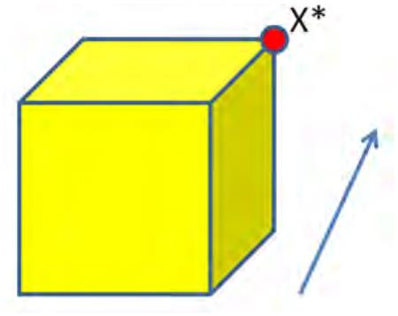

In an iteration of the simplex method, the current vertex may have multiple neighboring
vertices with better objective function value. The choice of which of these to move to is
known as a pivot rule.
2
.2.3 Correctness
The simplex method is guaranteed to terminate at an optimal solution.7 The intuition for
this fact should be clear from Figure 1 — since the objective function is linear and the
feasible region is convex, if no “local move” from a vertex is improving, then there should
be no direction at all within the feasible region that leads to a better solution. Formally,
the simplex method “knows that it’s done” by, at termination, exhibiting a a feasible dual
solution such that the complementary slackness conditions hold (see Lecture #9). Indeed,
the proof that the simplex method is guaranteed to terminate with an optimal solution
provides another proof of strong LP duality.
In terms of our three-step design paradigm (Lecture #9), we can think of the simplex
method as maintaining primal feasibility and the complementary slackness conditions and
working toward dual feasibility.8
2
.2.4 Worst-Case Running Time
As mentioned, the simplex method is very fast in practice, and routinely solves linear pro-
grams with hundreds of thousands or even millions of variables and constraints. However,
it is a bizarre mathematical fact that the worst-case running time of the simplex method
is exponential in the input size. To understand the issue, first note that the number of
vertices of a feasible region can be exponential in the dimension (e.g., the 2n vertices of the
n-dimensional hypercube). Much harder is constructing a linear program where the simplex
method actually visits all of the vertices of the feasible region. Such an example was given
by Klee and Minty in the early 1970s (25 years after simplex has invented). Their example
is a “squashed” version of an n-dimensional hypercube. Such exponential lower bounds are
known for all natural deterministic pivot rules.9
The number of iterations required by the simplex method is also related to one of the most
famous open problems in combinatorial geometry, the Hirsch conjecture. This conjecture
concerns the “diameter of polytopes,” meaning the diameter of the graph derived from the
with equality. (E.g., in the plane, this would be 3 constraints whose boundaries meet at a common point.)
In this case, a constraint swap can result in staying at the same vertex. There are simple ways to avoid
cycling, however, which we won’t discuss here.
7
Assuming that the linear program is feasible and has a finite optimum. If not, the simplex method
correctly detects which of these cases the linear program falls in.
How does the simplex method find the initial primal feasible point? For some linear programs this is
8
easy (e.g., the all-0 vector is feasible). In general, one can an additional variable, highly penalized in the
objective function, to make finding an initial feasible point trivial.
9
Interestingly, some randomized pivot rules (e.g., among the neighboring vertices that are better, pick one
at random) require, in expectation, at most ≈ 2 n iterations to converge on every instance. There are now
√
nearly matching upper and lower bounds on the required number of iterations for all the natural randomized
rules.
7


skeleton of the polytope (with vertices and edges of the polytope inducing, um, vertices
and edges of the graph). The conjecture asserts that the diameter is always at most linear
(in the number of variables and constraints). The best known upper bound on the worst-
case diameter of polytopes is “quasi-polynomial” (of the form ≈ nlog n), due to Kalai and
Kleitman in the early 1990s. Since the trajectory of the simplex method is a walk along the
edges of the feasible region, the number of iterations required (for a worst-case starting point
and objective function) is at least the polytope diameter. Put differently, sufficiently good
upper bounds on the number of iterations required by the simplex method (for some pivot
rule) would automatically yield progress on the Hirsch conjecture.
2
.2.5 Average-Case and Smoothed Running Time
The worst-case running time of the wildly practical simplex method poses a real quandary
for the mathematical analysis of algorithms. Can we “correct” the theory so that it better
reflects reality?
In the 1980s, a number of researchers (Borgwardt, Smale, Adler-Karp, etc.) showed that
the simplex method (with a suitable pivot rule) runs in polynomial time “on average” with
respect to various distributions over linear programs. Note that it is not at all obvious how
to define a “random linear program.” Indeed, many natural attempts lead to linear programs
that are almost always infeasible.
At the start of the 21st century, Spielman and Teng proved that the simplex method has
polynomial “smoothed complexity.” This is like a robust version of an average-cases analysis.
The model is to take a worst-case initial linear program, and then to randomly perturb it a
small amount. The main result here is that, for every initial linear program, in expectation
over the perturbed version of the linear program, the running time of simplex is polynomial
in the input size. The take-away being that bad examples for the simplex method are both
rare and isolated, in a precise sense. See the instructor’s CS264 course (“Beyond Worst-Case
Analysis”) for much more on smoothed analysis.
2
.3 The Ellipsoid Method
2
.3.1 Worst-Case Running Time
The ellipsoid method was originally proposed (by Shor and others) in the early/mid-1970s
as an algorithm for nonlinear programming. In 1979 Khachiyan proved that, for linear
programs, the algorithm is actually guaranteed to run in polynomial time. This was the
first-ever polynomial-time algorithm for linear programming, a big enough deal at the time
to make the front page of the New York Times (if below the fold).
The ellipsoid method is very slow in practice — usually multiple orders of magnitude
slower than the fastest methods. How can a polynomial-time algorithm be so much worse
than the exponential-time simplex method? There are two issues. First, the degree in
the polynomial bounding the ellipsoid method’s running time is pretty big (like 4 or 5,
depending on the implementation details). Second, the performance of the ellipsoid method
8
on “typical cases” is generally close to its worst-case performance. This is in sharp contrast
to the simplex method, which almost always solves linear programs in time far less than its
worst-case (exponential) running time.
2
.3.2 Separation Oracles
Figure 2: The responsibility of a separation oracle.
The ellipsoid method is uniquely useful for proving theorems — for establishing that other
problems are worst-case polynomial-time solvable, and thus are at least efficiently solvable
in principle. The reason is that the ellipsoid method can solve some linear programs with
n variables and an exponential (in n) number of constraints in time polynomial in n. How
is this possible? Doesn’t it take exponential time just to read in all of the constraints?
For other linear programming algorithms, yes. But the ellipsoid method doesn’t need an
explicit description of the linear program — all it needs is a helper subroutine known as a
separation oracle. The responsibility of a separation oracle is to take as input an allegedly
feasible solution x to a linear program, and to either verify feasibility (if x is indeed feasible)
or produce a constraint violated by x (otherwise). See Figure 2. Of course, the separation
oracle should also run in polynomial time.10
How could one possibly check an exponential number of constraints in polynomial time?
You’ve actually already seen some examples of this. For example, recall the dual of the
path-based linear programming formulation of the maximum flow problem (Lecture #8):
X
min
u `
e e
e∈E
1
0Such separation oracles are also useful in some practical linear programming algorithms: in “cutting
plane methods,” for linear programs with a large number of constraints (where the oracle is used in the
same way as in the ellipsoid method); and in the simplex method for linear programs with a large number of
variables (where the oracle is used to generate variables on the fly, a technique called “column generation”).
9
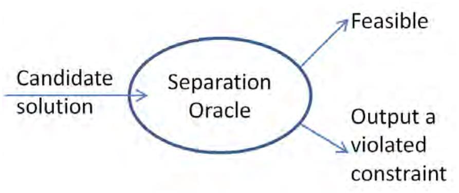

subject to
X
`e ≥ 1
`e ≥ 0
for all P ∈ P
for all e ∈ E.
(6)
e∈P
Here P denotes the set of s-t flow paths of a maximum flow instance (with edge capacities
u ). Since a graph can have an exponential number of s-t paths, this linear program has a
e
potentially exponential number of constraints.11 But, it has a polynomial-time separation
oracle. The key observation is: at least one constraint is violated if and only if
X
min
P∈P
`e < 1.
e∈P
Thus, the separation oracle is just Dijkstra’s algorithm! In detail: given an allegedly feasible
solution {` }
to the linear program, the separation oracle first checks that each `e is
e
e∈E
nonnegative (if ` < 0, it returns the violated constraint ` ≥ 0). If the solution passes this
e
e
test, then the separation oracle runs Dijkstra’s algorithm to compute a shortest s-t path,
using the `e’s as (nonnegative) edge lengths. If the shortest path has length at least 1, then
all of the constraints (6) are satisfied and the oracle reports “feasible.” If the shortest path
P
P∗ has length less than 1, then it returns the violated constraint
can solve the above linear program in polynomial time using the ellipsoid method.12
`e
≥
1. Thus, we
e∈P∗
2
.3.3 How the Ellipsoid Method Works
Here is a sketch of how the ellipsoid method works. The first step is to reduce optimization
to feasibility. That is, if the objective is max cT x, one replaces the objective function by
the constraint cT x ≥ M for some target objective function value M. If one can solve this
feasibility problem in polynomial time, then one can solve the original optimization problem
using binary search on the target objective M.
There’s a silly story about how to hunt a lion in the Sahara. The solution goes: encircle
the Sahara with a high fence and then bifurcate it with another fence. Figure out which side
has the lion in it (e.g., looking for tracks), and recurse. Eventually, the lion is trapped in
such a small area that you know exactly where it is.
1
1For example, consider the graph s = v , v , . . . , v = t, with two parallel edges directed from each v to
1
2
n
i
vi+1
.
1
2Of course, we already know how to solve this particular linear program in polynomial time — just
compute a minimum s-t cut (see Lecture #8). But there are harder problems where the only known proof
of polynomial-time solvability goes through the ellipsoid method.
1
0

Figure 3: The ellipsoid method first initializes a huge sphere (blue circle) that encompasses
the feasible region (yellow pentagon). If the ellipsoid center is not feasible, the separation
oracle produces a violated constraint (dashed line) that splits the ellipsoid into two regions,
one containing the feasible region and one that does not. A new ellipsoid (red oval) is drawn
that contains the feasible half-ellipsoid, and the method continues recursively.
Believe it or not, this story is a pretty good cartoon of how the ellipsoid method works.
The ellipsoid method maintains at all times an ellipsoid which is guaranteed to contain the
entire feasible region (Figure 3). It starts with a huge sphere to ensure the invariant at
initialization. It then invokes the separation oracle on the center of the current ellipsoid.
If the ellipsoid center is feasible, then the problem is solved. If not, the separation oracle
produces a constraint satisfied by all feasible points that is violated by the ellipsoid center.
Geometrically, the feasible region and the ellipsoid center are on opposite sides of the corre-
sponding halfspace boundary (Figure 3). Thus we know we can recurse on the appropriate
half-ellipsoid. Before recursing, however, the ellipsoid method redraws a new ellipsoid that
contains this half-ellipsoid (and hence the feasible region).13 Elementary but tedious calcu-
lations show that the volume of the current ellipsoid is guaranteed to shrink at a certain rate
at each iteration, and this yields a polynomial bound on the number of iterations required.
The algorithm stops when the current ellipsoid is so small that it cannot possibly contain a
feasible point (given the precision of the input data).
Now that we understand how the ellipsoid method works at a high level, we see why it
can solve linear programs with an exponential number of constraints. It never works with an
explicit description of the constraints, and just generates constraints on the fly on a “need
to know” basis. Because it terminates in a polynomial number of iterations, it only ever
1
3Why the obsession with ellipsoids? Basically, they are the simplest shapes that can decently approximate
all shapes of polytopes (“fat” ones, “skinny” one, etc.). In particular, every ellipsoid has a well defined and
easy-to-compute center.
1
1
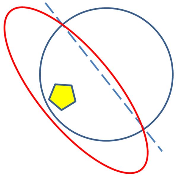

generates a polynomial number of constraints.14
2
.4 Interior-Point Methods
While the simplex method works “along the boundary” of the feasible region, and the ellip-
soid method works “outside in,” the third and again quite different paradigm of interior-point
methods works “inside out.” There are many genres of interior-point methods, beginning
with Karmarkar’s algorithm in 1984 (which again made the New York Times, this time
above the fold). Perhaps the most popular are “central path” methods. The idea is, instead
of maximizing the given objective cT x, to maximize
T
c x − λ · f(distance between x and boundary),
barrier function
|
{z
}
where λ ≥ 0 is a parameter and f is a “barrier function” that blows up (to +∞) as its
1
argument goes to 0 (e.g., log ). Initially, one sets λ so big that the problem become easy
1
z
(when f(x) = log , the solution is the “analytic center” of the feasible region, and can
z
be computed using e.g. Newton’s method). Then one gradually decreases the parameter λ,
tracking the corresponding optimal point along the way. (The “central path” is the set of
optimal points as λ varies from ∞ to 0.) When λ = 0, the optimal point is an optimal
solution to the linear program, as desired.
The two things you should know about interior-point methods are: (i) many such algo-
rithms run in time polynomial in the worst case; and (ii) such methods are also competitive
with the simplex method in practice. For example, one of Matlab’s LP solvers uses an
interior-point algorithm.
There are many linear programs where interior-point methods beat the best simplex codes
(especially on larger LPs), but also vice versa. There is no good understanding of when one
is likely to outperform the other. Despite the fact that it’s 70 years old, the simplex method
remains the most commonly used linear programming algorithm in practice.
1
4As a sanity check, recall that every vertex of a feasible region in Rn is the unique point satisfying some
subset of n constraints with equality. Thus in principle there’s always n constraints the are sufficient to
describe one feasible point (given a separation oracle to verify feasibility). The magic of the ellipsoid method
is that, even though a priori it has no idea which subset of constraints is the right one, it always finds a
feasible point while generating only a polynomial number of constraints.
1
2


CS261: A Second Course in Algorithms
Lecture #11: Online Learning and the Multiplicative
Weights Algorithm∗
Tim Roughgarden†
February 9, 2016
1
Online Algorithms
This lecture begins the third module of the course (out of four), which is about online
algorithms. This term was coined in the 1980s and sounds anachronistic there days — it has
nothing to do with the Internet, social networks, etc. It refers to computational problems of
the following type:
An Online Problem
1
2
. The input arrives “one piece at a time.”
. An algorithm makes an irrevocable decision each time it receives a new
piece of the input.
For example, in job scheduling problems, one often thinks of the jobs as arriving online (i.e.,
one-by-one), with a new job needing to be scheduled on some machine immediately. Or in a
graph problem, perhaps the vertices of a graph show up one by one (with whatever edges are
incident to previously arriving vertices). Thus the meaning of “one piece at a time” varies
with the problem, but it many scenarios it makes perfect sense. While online algorithms
don’t get any airtime in an introductory course like CS161, many problems in the real world
(computational and otherwise) are inherently online problems.
∗
†
ꢀc
2
Department of Computer Science, Stanford University, 474 Gates Building, 353 Serra Mall, Stanford,
016, Tim Roughgarden.
CA 94305. Email: tim@cs.stanford.edu.
1


2
Online Decision-Making
2
.1 The Model
Consider a set A of n ≥ 2 actions and a time horizon T ≥ 1. We consider the following
setup.
Online Decision-Making
At each time step t = 1, 2, . . . , T:
a decision-maker picks a probability distribution pt over her actions
A
an adversary picks a reward vector rt : A → [−1, 1]
an action at is chosen according to the distribution pt, and the
decision-maker receives reward rt(at)
the decision-maker learns rt, the entire reward vector
An online decision-making algorithm specifies for each t the probability distribution pt,
as a function of the reward vectors r1, . . . , rt−1 and realized actions a1, . . . , at−1 of the first
t − 1 time steps. An adversary for such an algorithm A specifies for each t the reward
vector rt, as a function of the probability distributions p1, . . . , pt used by A on the first t
days and the realized actions a1, . . . , at of the first t 1 days.
−
1
−
For example, A could represent different investment strategies, different driving routes
between home and work, or different strategies in a zero-sum game.
2
.2 Definitions and Examples
We seek a “good” online decision-making algorithm. But the setup seems a bit unfair, no?
The adversary is allowed to choose each reward function rt after the decision-maker has
committed to her probability distribution pt. With such asymmetry, what kind of guarantee
can we hope for? This section gives three examples that establish limitations on what is
possible.1
The first example shows that there is no hope of achieving reward close to that of the
P
T
t=1
maxa∈A rt(a) is just too strong.
best action sequence in hindsight. This benchmark
Example 2.1 (Comparing to the Best Action Sequence) Suppose A = {1, 2} and fix
an arbitrary online decision-making algorithm. Each day t, the adversary chooses the reward
vector rt as follows: if the algorithm chooses a distribution pt for which the probability on
action 1 is at least , then r is set to the vector ( 1, 1). Otherwise, the adversary sets r equal
t
1
2
−
t
1
In the first half of the course, we always sought algorithms that are always correct (i.e., optimal). In an
online setting, where you have to make decisions without knowing the future, we expect to compromise on
an algorithm’s guarantee.
2


to (1, −1). This adversary forces the expected reward of the algorithm to be nonpositive,
while ensuring that the reward of the best action sequence in hindsight is T.
Example 2.1 motivates the following important definitions. Rather than comparing the
expected reward of an algorithm to that of the best action sequence in hindsight, we compare
it to the reward incurred by the best fixed action in hindsight. In words, we change our
P
P
T
t=1
maxa∈A rt(a) to maxa∈A
T
t=1
rt(a).
benchmark from
Definition 2.2 (Regret) Fix reward vectors r1, . . . , rT . The regret of the action sequence
a1, . . . , aT is
XT
best fixed action
XT
our algorithm
t
t
r (a ) .
max
a∈A
rt(a) −
(1)
t=1
t=1
|
{z
}
|
{z
}
We’d like an online decision-making algorithm that achieves low regret, as close to 0 as
possible (and negative regret would be even better).2 Notice that the worst-possible regret
in 2T (since rewards lie in [−1, 1]). We think of regret Ω(T) as an epic fail for an algorithm.
What is the justification for the benchmark of the best fixed action in hindsight? First,
simple and natural learning algorithms can compete with this benchmark. Second, achieving
this is non-trivial: as the following examples make clear, some ingenuity is required. Third,
competing with this benchmark is already sufficient to obtain many interesting applications
(see end of this lecture and all of next lecture).
One natural online decision-making algorithm is follow-the-leader , which at time step t
t−1
chooses the action a with maximum cumulative reward
P
ru(a) so far. The next example
shows that follow-the-leader, and more generally every deterministic algorithm, can have
regret that grows linearly with T.
u=1
Example 2.3 (Randomization Is Necessary for No Regret) Fix a deterministic on-
line decision-making algorithm. At each time step t, the algorithm commits to a single
action at. The obvious strategy for the adversary is to set the reward of action at to 0, and
the reward of every other action to 1. Then, the cumulative reward of the algorithm is 0
while the cumulative reward of the best action in hindsight is at least T(1 − ). Even when
1
n
there are only 2 actions, for arbitrarily large T, the worst-case regret of the algorithm is at
T
least .
2
For randomized algorithms, the next example limits the rate at which regret can vanish
as the time horizon T grows.
p
Example 2.4 ( (ln n)/T Regret Lower Bound) Suppose there are n = 2 actions, and
that we choose each reward vector rt independently and equally likely to be (1, −1) or (−1, 1).
No matter how smart or dumb an online decision-making algorithm is, with respect to this
random choice of reward vectors, its expected reward at each time step is exactly 0 and its
2
Sometimes this goal is referred to as “combining expert advice” — if we think of each action as an
expert,” then we want to do as well as the best expert.
“
3


expected cumulative reward is thus also 0. The expected cumulative reward of the best fixed
action in hindsight is b T, where b is some constant independent of T. This follows from
√
T
2
the fact that if a fair coin is flipped T times, then the expected number of heads is and
√
1
2
the standard deviation is
T.
Fix an online decision-making algorithm A. A random choice of reward vectors causes A
√
to experience expected regret at least b T, where the expectation is over both the random
choice of reward vectors and the action realizations. At least one choice of reward vec-
tors induces an adversary that causes A to have expected regret at least b T, where the
√
expectation is over the action realizations.
A similar argument shows that, with n actions, the expected regret of an online decision-
√
making algorithm cannot grow more slowly than b T ln n, where b > 0 is some constant
independent of n and T.
3
The Multiplicative Weights Algorithm
We now give a simple and natural algorithm with optimal worst-case expected regret, match-
ing the lower bound in Example 2.4 up to constant factors.
Theorem 3.1 There is an online decision-making algorithm that, for every adversary, has
expected regret at most 2 T ln n.
√
An immediately corollary is that the number of time steps needed to drive the expected
time-averaged regret down to a small constant is only logarithmic in the number of actions.3
Corollary 3.2 There is an online decision-making algorithm that, for every adversary and
ꢀ
> 0, has expected time-averaged regret at most ꢀ after at most (4 ln n)/ꢀ2 time steps.
In our applications in this and next lecture, we will use the guarantee in the form of Corol-
lary 3.2.
The guarantees of Theorem 3.1 and Corollary 3.2 are achieved by the multiplicative
weights (MW) algorithm.4 Its design follows two guiding principles.
No-Regret Algorithm Design Principles
1
. Past performance of actions should guide which action is chosen at each
time step, with the probability of choosing an action increasing in its
cumulative reward. (Recall from Example 2.3 that we need a randomized
algorithm to have any chance.)
3
4
Time-averaged regret just means the regret, divided by T.
This and closely related algorithms are sometimes called the multiplicative weight update (MWU) algo-
rithm, Polynomial Weights, Hedge, and Randomized Weighted Majority.
4


2
. The probability of choosing a poorly performing action should decrease
at an exponential rate.
The first principle is essential for obtaining regret sublinear in T, and the second for optimal
regret bounds.
The MW algorithm maintains a weight, intuitively a “credibility,” for each action. At
each time step the algorithm chooses an action with probability proportional to its cur-
rent weight. The weight of each action evolves over time according to the action’s past
performance.
Multiplicative Weights (MW) Algorithm
initialize w1(a) = 1 for every a ∈ A
for each time step t = 1, 2, . . . , T do
use the distribution pt := wt/Γt over actions, where
P
Γt =
wt(a) is the sum of the weights
a∈A
given the reward vector rt, for every action a ∈ A use the formula
wt+1(a) = wt(a) · (1 + ηrt(a)) to update its weight
For example, if all rewards are either -1 or 1, then the weight of each action a either goes up
by a 1 + η factor or down by a 1 − η factor. The parameter η lies between 0 and , and is
1
2
chosen at the end of the proof of Theorem 3.1 as a function of n and T. For intuition, note
that when η is close to 0, the distributions pt will hew close to the uniform distribution.
Thus small values of η encourage exploration. Large values of η correspond to algorithms
in the spirit of follow-the-leader. Thus large values of η encourage exploitation, and η is a
knob for interpolating between these two extremes. The MW algorithm is obviously simple
to implement, since the only requirement is to update the weight of each action at each time
step.
4
Proof of Theorem 3.1
Fix a sequence r1, . . . , rT of reward vectors.5 The challenge is that the two quantities that
we care about, the expected reward of the MW algorithm and the reward of the best fixed
action, seem to have nothing to do with each other. The fairly inspired idea is to relate both
P
of these quantities to an intermediate quantity, namely the sum ΓT+1 =
the actions’ weights at the conclusion of the MW algorithm. Theorem 3.1 then follows from
some simple algebra and approximations.
wT+1(a) of
a∈A
5
We’re glossing over a subtle point, the difference between “adaptive adversaries” (like those defined in
Section 2) and “oblivious adversaries” which specify all reward vectors in advance. Because the behavior of
the MW algorithm is independent of the realized actions, it turns out that the worst-case adaptive adversary
for the algorithm is in fact oblivious.
5


The first step, and the step which is special to the MW algorithm, shows that the sum
of the weights Γt evolves together with the expected reward earned by the MW algorithm.
In detail, denote the expected reward of the MW algorithm at time step t by νt, and write
X
X
wt(a)
νt =
p (a) · r (a) =
t
t
· rt(a).
(2)
Γt
a∈A
a∈A
Thus we want to lower bound the sum of the νt’s.
To understand Γt+1 as a function of Γt and the expected reward (2), we derive
X
Γt+1
=
wt+1(a)
a∈A
X
t
t
=
=
w (a) · (1 + ηr (a))
a∈A
Γ (1 + ην ).
t
t
(3)
For convenience, we’ll bound from above this quantity, using the fact that 1 + x ≤ ex for all
real-valued x.6 Then we can write
Γt+1 ≤ Γt · eηνt
for each t and hence
YT
P
eηνt = n · eη
T
t=1
νt
.
(4)
ΓT+1 ≤ Γ
1
|
{z}
=
n
t=1
This expresses a lower bound on the expected reward of the MW algorithm as a relatively
simple function of the intermediate quantity ΓT+1.
Figure 1: 1 + x ≤ ex for all real-valued x.
6
See Figure 1 for a proof by picture. A formal proof is easy using convexity, a Taylor expansion, or other
methods.
6

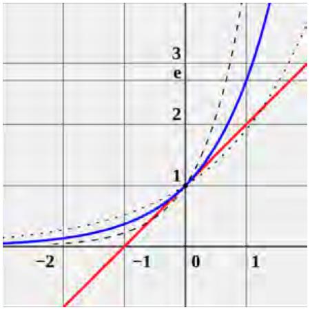

The second step is to show that if there is a good fixed action, then the weight of this
action single-handedly shows that the final value ΓT+1 is pretty big. Combining with the
first step, this will imply the the MW algorithm only does poorly if every fixed action is bad.
P
T
t=1
t
∗
r (a ) of the best fixed action a
∗
Formally, let OPT denote the cumulative reward
for the reward vector sequence. Then,
ΓT+1 ≥ wT+1(a∗)
YT
1
∗
w (a ) (1 + ηr (a )).
t
∗
=
(5)
|
{z }
t=1
=
1
OPT is the sum of the rt(a )’s, so we’d like to massage the expression above to involve this
sum. Products become sums in exponents. So the first idea is to use the same trick as before,
replacing 1 + x by ex. Unfortunately, we can’t have it both ways — before we wanted an
upper bound on 1 + x, whereas now we want a lower bound. But looking at Figure 1, it’s
clear that the two function are very close to each other for x near 0. This can made precise
through the Taylor expansion
∗
x2
2
x3 − x4
ln(1 + x) = x −
+
+
· · ·
.
3
4
Provided |x| ≤ , we can obtain a lower bound on ln(1 + x) by throwing out all terms but
1
2
the first two, and doubling the second term to compensate. (The magnitudes of the rest of
x2
2
1
2
1
4
−x22
the terms can be bounded above by the geometric series ( + +
term blows them all away.)
· · ·
), so the extra
Since η ≤ and r (a )
1
2
| t ∗ | ≤
1 for every t, we can plug this estimate into (5) to obtain
YT
ΓT+1
ηrt(a∗)−
η (r (a ))
2
t
∗
2
≥
≥
e
t=1
ηOPT−η2T
e
,
(6)
where in (6) we’re just using the crude estimate (rt(a∗))
Through (4) and (6), we’ve connected the cumulative expected reward
2 ≤
1 for all t.
P
T
t=1
νt of the
MW algorithm with the reward OPT of the best fixed auction through the intermediate
quantity ΓT+1:
P
and hence (taking the natural logarithm of both sides and dividing through by η):
T
t=1
νt
≥ ΓT+1 ≥ eηOPT−η2T
n · eη
XT
ln n
νt ≥ OPT − ηT −
.
(7)
η
t=1
Finally, we set the free parameter η. There are two error terms in (7), the first one corre-
sponding to inaccurate learning (higher for larger learning rates), the second corresponding
to overhead before converging (higher for smaller learning rates). To equalize the two terms,
7


p
fixed action. This completes the proof of Theorem 3.1.
1
we choose η = (ln n)/T. (Or η = , if this is smaller.) Then, the cumulative expected
2
√
reward of the MW algorithm is at most 2 T ln n less than the cumulative reward of the best
Remark 4.1 (Unknown Time Horizons) The choice of η above assumes knowledge of
the time horizon T. Minor modifications extend the multiplicative weights algorithm and
its regret guarantee to the case where T is not known a priori, with the “2” in Theorem 3.1
replaced by a modestly larger constant factor.
5
Minimax Revisited
Recall that a two-player zero-sum game can be specified by an m × n matrix A, where a
ij
denotes the payoff of the row player and the negative payoff of the column player when row i
and column j are chosen. It is easy to see that going first in a zero-sum game can only be
worse than going second — in the latter case, a player has the opportunity to adapt to the
first player’s strategy. Last lecture we derived the minimax theorem from strong LP duality.
It states that, provided the players randomize optimally, it makes no difference who goes
first.
Theorem 5.1 (Minimax Theorem) For every two-player zero-sum game A,
ꢀ
ꢁ
ꢂ
ꢃ
>
>
max min x Ay = min max x Ay .
(8)
x
y
y
x
We next sketch an argument for deriving Theorem 5.1 directly from the guarantee pro-
vided by the multiplicative weights algorithm (Theorem 3.1). Exercise Set #6 asks you to
provide the details.
Fix a zero-sum game A with payoffs in [−1, 1] and a value for a parameter ꢀ > 0. Let
n denote the number of rows or the number of columns, whichever is larger. Consider the
following thought experiment:
•
At each time step t = 1, 2, . . . , T = 4 ln n:
ꢀ
2
–
–
–
The row and column players each choose a mixed strategy (pt and qt, respectively)
using their own copies of the multiplicative weights algorithm (with the action set
equal to the rows or columns, as appropriate).
The row player feeds the reward vector rt = Aqt into (its copy of) the multiplica-
tive weights algorithm. (This is just the expected payoff of each row, given that
the column player chose the mixed strategy qt.)
Analogously, the column player feeds the reward vector rt = −(pt)T A into the
multiplicative weights algorithm.
8


Let
XT
1
t T
(p ) Aq
t
v =
T
t=1
denote the time-averaged payoff of the row player. The first claim is that applying Theo-
rem 3.1 (in the form of Corollary 3.2) to the row and column players implies that
ꢀ
ꢁ
T
v ≥ max p Aqˆ − ꢀ
p
and
ꢀ
ꢁ
T
v ≤ min pˆ Aq + ꢀ,
q
P
P
1
T
T
t=1
pt and qˆ =
1
T
T
t=1
qt denote the time-averaged row and
respectively, where pˆ =
column strategies.
Given this, a short derivation shows that
ꢀ
ꢁ
ꢀ
ꢁ
T
T
max min p Aq ≥ min min p Aq − 2ꢀ.
p
q
q
p
Letting ꢀ → 0 and recalling the easy direction of the minimax theorem (max min p Aq
>
≤
p
q
>
min max p Aq) completes the proof.
q
p
9


CS261: A Second Course in Algorithms
Lecture #12: Applications of Multiplicative Weights to
Games and Linear Programs∗
Tim Roughgarden†
February 11, 2016
1
Extensions of the Multiplicative Weights Guarantee
Last lecture we introduced the multiplicative weights algorithm for online decision-making.
You don’t need to remember the algorithm details for this lecture, but you should remember
that it’s a simple and natural algorithm (just one simple update per action per time step).
You should also remember its regret guarantee, which we proved last lecture and will use
today several times as a black box.1
Theorem 1.1 The expected regret of the multiplicative weights algorithm is always at most
T ln n, where n is the number of actions and T is the time horizon.
√
2
Recall the definition of regret, where A denotes the action set:
XT
best fixed action
XT
our algorithm
t
r (a ) .
t
max
a∈A
rt(a) −
t=1
{z
t=1
|
}
|
{z
}
The expectation in Theorem 1.1 is over the random choice of action in each time step; the
reward vectors r1, . . . , rT are arbitrary.
The regret guarantee in Theorem 1.1 applies not only with with respect to the best
fixed action in hindsight, but more generally to the best fixed probability distribution in
∗
†
ꢀc
2
Department of Computer Science, Stanford University, 474 Gates Building, 353 Serra Mall, Stanford,
016, Tim Roughgarden.
CA 94305. Email: tim@cs.stanford.edu.
This lecture is a detour from our current study of online algorithms. While the multiplicative weights
algorithm works online, the applications we discuss today are not online problems.
1
1


hindsight. The reason is that, in hindsight, the best fixed action is as a good as the best
fixed distribution over actions. Formally, for every distribution p over A,
!
XT X
X
XT
XT
t
rt(a) ≤ max
rt(b).
p · r (a) =
p
a
a
|
{z}
b∈A
t=1 a∈A
a∈A
t=1
t=1
sum to 1 |
{z
}
P
We’ll apply Theorem 1.1 in the following form (where time-averaged just means divided
≤
maxb
rt(b)
t
by T).
Corollary 1.2 The expected time-averaged regret of the multiplicative weights algorithm is
at most ꢀ after at most (4 ln n)/ꢀ2 time steps.
As noted above, the guarantee of Corollary 1.2 applies with respect to any fixed distribution
over the actions.
Another useful extension is to rewards that lie in [−M, M], rather than in [−1, 1]. This
scenario reduces to the previous one by scaling. To obtain time-averaged regret at most ꢀ:
1
2
. scale all rewards down by M;
. run the multiplicative weights algorithm until the time-averaged expected regret is at
ꢀ
M
most
;
3
. scale everything back up.
Equivalently, rather than explicitly scaling the reward vectors, one can change the weight
update rule from wt+1(a) = wt(a)(1 + ηrt(a)) to wt+1(a) = wt(a)(1 + rt(a)). In any case,
η
M
iterations, the time-averaged expected regret is
4
M2 ln n
Corollary 1.2 implies that after T =
at most ꢀ.
ꢀ
2
2
Minimax Revisited (Again)
Last lecture we sketched how to use the multiplicative weights algorithm to prove the min-
imax theorem (details on Exercise Set #6). The idea was to have both the row and the
column player play a zero-sum game repeatedly, using their own copies of the multiplicative
weights algorithm to choose strategies simultaneously at each time step. We next discuss an
alternative thought experiment, where the players move sequentially at each time step with
only the row player using multiplicative weights (the column player just best responds). This
alternative has similar consequences and translates more directly into interesting algorithmic
applications.
Fix a zero-sum game A with payoffs in [−M, M] and a value for a parameter ꢀ > 0. Let
m denote the number of rows of A. Consider the following thought experiment, in which
the row player has to move first and the column player gets to move second:
2


Thought Experiment
•
At each time step t = 1, 2, . . . , T = 4M2
ln m
2
:
ꢀ
–
–
–
The row player chooses a mixed strategy pt using the multiplicative
weights algorithm (with the action set equal to the rows).
The column player responds optimally with the deterministic strat-
egy qt.2
If the column player chooses column j, then set rt(i) = aij for every
row i, and feed the reward vector rt into the multiplicative weights
algorithm. (This is just the payoff of each row in hindsight, given
the column player’s strategy at time t.)
We claim that the column player get at least its minimax payoff, and the row player gets
at least its minimax payoff minus ꢀ.
Claim 1: In the thought experiment above, the negative time-averaged expected payoff of
the column player is at most
ꢀ
ꢁ
T
max min p Aq .
p
q
Note that the benchmark used in this claim is the more advantageous one for the column
player, where it gets to move second.3
Proof: The column player only does better than its minimax value because, not only does
the player get to go second, but the player can tailor its best responses on each day to
P
1
T
t=1
pt denote the
the row player’s mixed strategy on that day. Formally, we let pˆ =
T
time-averaged row strategy and q an optimal response to p and derive
∗
ˆ
ꢀ
ꢁ
T
T
max min p Aq ≥ min pˆ Aq
p
q
q
=
pˆT Aq∗
XT
1
t T
(p ) Aq∗
=
T
t=1
XT
1
t T
(p ) Aq ,
t
≥
T
t=1
with the the last inequality following because qt is an optimal response to pt for each t.
(Recall the column player wants to minimize pT Aq.) Since the last term is the negative
2
Recall from last lecture that the player who goes second has no need to randomize: choosing a column
with the best expected payoff (given the row player’s strategy pt) is the best thing to do.
Of course, we’ve already proved the minimax theorem, which states that it doesn’t matter who goes
3
first. But here we want to reprove the minimax theorem, and hence don’t want to assume it.
3


time-averaged payoff of the column player in the thought experiment, the proof is complete.
ꢀ
Claim 2: In the thought experiment above, the time-averaged expected payoff of the row
player is at least
ꢀ
We are again using the stronger benchmark from the player’s perspective, here with the row
ꢁ
T
min max p Aq − ꢀ.
q
p
player going second.
P
1
T
T
t=1
qt denote the time-averaged column strategy. The multiplicative
Proof: Let qˆ =
weights guarantee, after being extended as in Section 1, states that the time-averaged ex-
pected payoff of the row player is within ꢀ of what it could have attained using any fixed
mixed strategy p. That is,
!
XT
XT
1
1
t T
t
pT Aqt − ꢀ
(p ) Aq ≥ max
T
T
p
t=1
t=1
T
=
max p Aqˆ − ꢀ
p
ꢀ
ꢁ
T
≥
min max p Aq − ꢀ.
q
p
ꢀ
Letting ꢀ → 0, Claims 1 and 2 provide yet another proof of the minimax theorem.
(Recalling the “easy direction” that max min pT Aq ≤ min max pT Aq.) The next order
p
q
q
q
of business is to translate this thought experiment into fast algorithms for approximately
solving linear programs.
3
Linear Classifiers Revisited
3
.1 Recap
Recall from Lecture #7 the problem of computing a linear classifier — geometrically, of
separating a bunch of “+”s and “-”s with a hyperplane (Figure 1).
4


Figure 1: We want to find a linear function that separates the positive points (plus signs)
from the negative points (minus signs)
Formally, the input consists of m “positive” data points p1, . . . , pm ∈ Rd and m “nega-
0
0
R
tive” data points q1, . . . , qm ∈ d. This corresponds to labeled data, with the positive and
negative points having labels +1 and -1, respectively.
The goal is to compute a linear function h(z) =
h(pi) > 0
P
d
j=1
Rd
to ) such that
R
a z + b (from
j
j
for all positive points and
h(qi) < 0
for all negative points. In Lecture #7 we saw how to compute a linear classifier (if one
exists) via linear programming. (It was almost immediate; the only trick was to introduce
an additional variable to turn the strict inequality constraints into the usual weak inequality
constraints.)
We’ve said in the past that linear programs with 100,000s of variables and constraints
are usually no problem to solve, and sometimes millions of variables and constraints are
also doable. But as you probably know from your other computer science courses, in many
cases we’re interested in considerably larger data sets. Can we compute a linear classifier
faster, perhaps under some assumptions and/or allowing for some approximation? The
multiplicative weights algorithm provides an affirmative answer.
3
.2 Preprocessing
We first execute a few preprocessing steps to transform the problem into a more convenient
form.
5
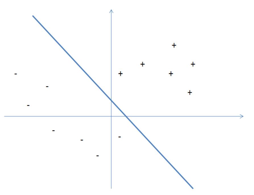
First, we can force the intercept b to be 0. The trick is to add an additional (d + 1)th
variable, with the new coefficient ad+1 corresponding to the old intercept b. Each positive
and negative data point gets a new (d + 1)th coordinate, equal to 1. Geometrically, we’re
now looking for a hyperplane separating the positive and negative points that passes through
the origin.
Second, if we multiply all the coordinates of each negative point yi ∈ Rd+1 by -1, then
we can write the constraints as
i
h(x ), h(y ) > 0
i
for all positive and negative data points. (For this reason, we will no longer distinguish
positive and negative points.) Geometrically, we’re now looking for a hyperplane (through
the origin) such that all of the data points are on the same side of the hyperplane.
Third, we can insist that every coefficient aj is nonnegative. (Don’t forget that the
coordinates of the xi’s can be both positive and negative.) The trick here is to make two
copies of every coordinate (blowing up the dimension from d + 1 to 2d + 2), and interpreting
0
j
00
j
the two coefficients a , a corresponding to the jth coordinate as indicating the coefficient
00
a = a0 a in the original space. For this to work, each entry x of a data point is replaced
−
i
j
j
j
j
by two entries, xi and −xi . Geometrically, we’re now looking for a hyperplane, through the
j
origin and with a normal vector in the nonnegative orthant, with all the data points on the
j
same side (and the same side as the normal vector).
For the rest of this section, we use d to denote the number of dimensions after all of this
preprocessing (i.e., we redefine d to be what was previously 2d + 2).
3
.3 Assumption
We assume that the problem is feasible — that there is a linear function of the desired type.
Actually, we assume a bit more, that there is a solution with some “wiggle room.”
Assumption: There is a coefficient vector a∗
∈ Rd
such that:
+
P
d
j=1
∗
i
1
2
.
.
a = 1; and
P
d
j=1
∗
i
for all data points xi.
a x >
ꢀ
|
{z}
j
j
“
margin”
Note that if there is any solution to the problem, then there is a solution satisfying the first
condition (just by scaling the coefficients). The second condition insists on wiggle room after
normalizing the coefficients to sum to 1.
Let M be such that |xij| ≤ M for every i and j. The running time of our algorithm will
depend on both ꢀ and M.
3
.4 Algorithm
Here is the algorithm.
6
1
2
. Define an action set A = {1, 2, . . . , d}, with actions corresponding to coordinates.
4
M2 ln d
. For t = 1, 2, . . . , T =
:
ꢀ
2
(a) Use the multiplicative weights algorithm to generate a probability distribution
at ∈ Rd over the actions/coordinates.
P
d
j=1
a x > 0 for every data point x , then halt and return a (which is a
i
t
i
t
(b) If
j
j
feasible solution).
P
(c) Otherwise, choose some data point xi with
d
j=1
a x ≤ 0, and define a reward
t
j
i
j
vector rt with rt(j) = xij for each coordinate j.
(d) Feed the reward vector rt into the multiplicative weights algorithm.
To motivate the choice of reward vector, suppose the coefficient vector at fails to have a
P
d
j=1
a x with the data point x . We want to nudge the coefficients
i
t
i
positive inner product
j
j
so that this inner product will go up in the next iteration. (Of course we might screw up
some other inner products, but we’re hoping it’ll work out OK in the end.) For coordinates j
with xi > 0 we want to increase a ; for coordinates with xi < 0 we want to do the opposite.
j
j
j
Recalling the multiplicative weight update rule (wt+1(a) = wt(a)(1 + ηrt(a))), we see that
the reward vector rt = xi will have the intended effect.
3
.5 Analysis
We claim that the algorithm above halts (necessarily with a feasible solution) by the time it
gets to the final iteration T.
In the algorithm, the reward vectors are nefariously defined so that, at every time step t,
the inner product of at and rt is non-positive. Viewing at as a probability distribution over
the actions {1, 2, . . . , d}, the means that the expected reward of the multiplicative weights
algorithm is non-positive at every time step, and hence its time-averaged expected reward
is at most 0.
On the other hand, by assumption (Section 3.3), there exists a coefficient vector (equiva-
lently, distribution over {1, 2, . . . , d}) a such that, at every time step t, the expected payoff
∗
P
P
∗
d
j=1
a r (j) min
t
∗
≥
m
i=1
d
j=1
∗
i
of playing a would have been
a x > ꢀ.
j
j
j
Combining these two observations, we see that as long as the algorithm has not yet
found a feasible solution, the time-averaged regret of the multiplicative weights subroutine
is strictly more than ꢀ. The multiplicative weights guarantee says that after T =
time-averaged regret is at most ꢀ.4 We conclude that our algorithm halts, with a feasible
linear classifier, within T iterations.
4
M2 ln d
, the
ꢀ
2
4
We’re using the extended version of the guarantee (Section 1), which holds against every fixed distribution
(like a∗) and not just every fixed action.
7


3
.6 Interpretation as a Zero-Sum Game
Our last two topics were a thought experiment leading to minimax payoffs in zero-sum games
and an algorithm for computing a linear classifier. The latter is just a special case of the
former.
To translate the linear classifier problem to a zero-sum game, introduce one row for each
of the d coordinates and one column for each of the data points xi. Define the payoff matrix
A by
ꢂ
ꢃ
i
j
A = a = x
ji
Recall that in our thought experiment (Section 2), the row player generates a strategy at
each time step using the multiplicative weights algorithm. This is exactly how we generate
the coefficient vectors a1, . . . , aT in the algorithm in Section 3.4. In the thought experiment,
the column player, knowing the row player’s distribution, chooses the column that minimizes
the expected payoff of the row player. In the linear classifier context, given at, this corre-
P
sponds to picking a data point xi that minimizes
d
j=1
a x . This ensures that a violated
t
i
j
j
data point (with nonpositive dot product) is chosen, provided one exists. In the thought
experiment, the reward vector rt fed into the multiplicative weights algorithm is the payoff of
each row in hindsight, given the column player’s strategy at time t. With the payoff matrix
A above, this vector corresponds to the data point xi chosen by the column player at time t.
These are exactly the reward vectors used in our algorithm for computing a linear classifier.
Finally, the assumption (Section 3.3) implies that the value of the constructed zero-sum
game is bigger than ꢀ (since the row player could always choose a∗). The regret guarantee
in Section 2 translates to the row player having time-averaged expected payoff bigger than
4
M2 ln m
0 once T exceeds
before this time.
. The algorithm has no choice but to halt (with a feasible solution)
ꢀ
2
4
Maximum Flow Revisited
4
.1 Multiplicative Weights and Linear Programs
We’ve now seen a concrete example of how to approximately solve a linear program using the
multiplicative weights algorithm, by modeling the linear program as a zero-sum game and
then applying the thought experiment from Section 2. The resulting algorithm is extremely
fast (faster than solving the linear program exactly) provided the margin ꢀ is not overly small
and the radius M of the ` ball enclosing all of the data points xij is not overly big.
∞
This same idea — associating one player with the decision variables and a second player
with the constraints — can be used to quickly approximate many other linear programs.
We’ll prove this point by considering one more example, our old friend the maximum flow
problem. Of course, we already know some pretty good algorithms (faster than linear pro-
grams) for maximum flow problems, but the ideas we’ll discuss extend also to multicom-
modity flow problems (see Exercise Set #6 and Problem Set #3), where we don’t know any
exact algorithms that are significantly faster than linear programming.
8

4
.2 A Zero-Sum Game for the Maximum Flow Problem
Recall the primal-dual pair of linear programs corresponding to the maximum flow and
minimum cut problems (Lecture #8):
X
max
fP
P∈P
subject to
X
fP ≤ 1
for all e ∈ E
P∈P : e∈P
|
{z
}
total flow on e
f ≥ 0
for all P ∈ P
P
and
X
min
`e
e∈E
subject to
X
`e ≥ 1
`e ≥ 0
for all P ∈ P
for all e ∈ E,
e∈P
where P denotes the set of s-t paths. To reduce notation, here we’ll only consider the case
where all edges have unit capacity (u = 1). The general case, with u ’s on the right-hand
e
e
side of the primal and in the objective function of the dual, can be solved using the same
ideas (Exercise Set #6).5
We begin by defining a zero-sum game. The row player will be associated with edges
(i.e., dual variables) and the column player with paths (i.e., primal variables). The payoff
matrix is
ꢄ
ꢅ
ꢆ
1
0
if e ∈ P
A = a
=
eP
otherwise
Note that all payoffs are 0 or 1. (Yes, this a huge matrix, but we’ll never have to write it
down explicitly; see the algorithm below.)
Let OPT denote the optimal objective function value of the linear programs. (The same
for each, by strong duality.) Recall that the value of a zero-sum game is defined as the
expected payoff of the row player under optimal play by both players (max min xT Ay or,
x
y
equivalently by the minimax theorem, min max xT Ay).
y
x
1
OPT
Claim: The value of this zero-sum game is
.
5
Although the running time scales quadratically with ratio of the maximum and minimum edge capacities,
which is not ideal. One additional idea (“width reduction”), not covered here, recovers a polynomial-time
algorithm for general edge capacities.
9


P
Proof: Let {`
∗
}
be an optimal solution to the dual, with
` = OPT. Obtain x ’s
∗
e
e
e∈E
e∈E
e
∗
from the ` ’s by scaling down by OPT — then the x ’s form a probability distribution. If the
e
row player uses this mixed strategy x, then each column P ∈ P results in expected payoff
e
X
X
1
1
∗
xe =
` ≥
,
e
OPT
OPT
e∈P
e∈P
where the inequality follows the dual feasibility of {` e∈E. This shows that the value of the
∗
e
}
1
OPT
game is at least
.
Conversely, let x be an optimal strategy for the row player, with min xT Ay equal to
y
the game’s value v. This means that, no matter what strategy the column player chooses,
the row player’s expected payoff is at least v. This translates to
X
xe ≥ v
e∈P
for every P ∈ P. Thus {x /v}
is a dual feasible solution, with objective function value
ꢀ
P
e
e∈E
1
OPT
(
x )/v = 1/v. Since this can only be larger than OPT, v ≤
.
e∈E
e
4
.3 Algorithm
For simplicity, assume that OPT is known.6 Translating the thought experiment from
Section 2 to this zero-sum game, we get the following algorithm:
1
2
. Associate an action with each edge e ∈ E.
4
OPT2 ln |E|
. For t = 1, 2, . . . , T =
:
ꢀ
2
(a) Use the multiplicative weights algorithm to generate a probability distribution
xt ∈ RE over the actions/edges.
(b) Let Pt be a column that minimizes the row player’s expected payoff (with the
expectation with respect to xt). That is,
X
t
t
e
P ∈ argmin
x .
(1)
P∈P
e∈P
(c) Define a reward vector rt with rt(e) = 1 for e ∈ Pt and rt(e) = 0 for e ∈/ Pt (i.e.,
the Ptth column of A). Feed the reward vector rt into the multiplicative weights
algorithm.
6
For example, embed the algorithm into an outer loop that uses successive doubling to “guess” the value
of OPT (i.e., take OPT = 1, 2, 4, 8, . . . until the algorithm succeeds).
1
0


4
.4 Running Time
An important observation is that this algorithm never explicitly writes down the payoff ma-
trix A. It maintains one weight per edge, which is a reasonable amount of state. To compute
Pt and the induced reward vector rt, all that is needed is a subroutine that solves (1) —
that, given the xt ’s, returns a shortest s-t path (viewing the xt ’s as edge lengths). Dijkstra’s
e
e
algorithm, for example, works just fine.7 Assuming Dijkstra’s algorithm is implemented in
O(m log n) time, where m and n denote the number of edges and vertices, respectively, the
OPT2
total running time of the algorithm is O(
m log m log n). (Note that with unit capacities,
ꢀ
2
OPT ≤ m. If there are no parallel edges, then OPT ≤ n − 1.) This is comparable to some
of the running times we saw for (exact) maximum flow algorithms, but more importantly
these ideas extend to more general problems, including multicommodity flow.
4
.5 Approximate Correctness
So how do we extract an approximately optimal flow from this algorithm? After running the
algorithm above, let P1, . . . , PT denote the sequence of paths chosen by the column player
(the same path can be chosen multiple times). Let ft denote the flow that routes OPT units
of flow on the path Pt. (Of course, this probably violates the edge capacity constraints.)
P
Finally, define f∗ =
1
T
T
t=1
ft as the “time-average” of these path flows. Note that since
each ft routes OPT units of flow from the source to the sink, so does f . But is f feasible?
∗
∗
Claim: f∗ routes at most 1 + ꢀ units of flow on every edge.
Proof: We proceed by contradiction. If f∗ routes more than 1+ꢀ units of flow on the edge e,
then more than (1 + ꢀ)T/OP T of the paths in P1, . . . , PT include the edge e. Returning to
our zero-sum game A, consider the row player strategy z that deterministically plays the
edge e. The time-averaged payoff to the row player, in hindsight given the paths chosen by
the column player, would have been
XT
X
1
1
1 + ꢀ
T
z Ay =
t
1 >
.
T
T
OPT
t=1
t : e∈Pt
The row player’s guarantee (Claim 1 in Section 2) then implies that
XT
But this contradicts the guarantee that the column player does at least as well as the minimax
XT
1
1
ꢀ
1 + ꢀ
ꢀ
1
t T
t
T
t
(x ) Ay ≥
z Ay −
>
−
=
.
T
T
OPT
OPT
OPT
OPT
t=1
t=1
1
OPT
ꢀ
value of the game (Claim 2 in Section 2), which is
by the Claim in Section 4.2.
Scaling down f∗ by a factor of 1+ꢀ yields a feasible flow with value at least OP T/(1+ꢀ).
7
This subroutine is precisely the “separation oracle” for the dual linear program, as discussed in Lecture
10 in the context of the ellipsoid method.
#
1
1


CS261: A Second Course in Algorithms
Lecture #13: Online Scheduling and Online Steiner Tree∗
Tim Roughgarden†
February 16, 2016
1
Preamble
Last week we began our study of online algorithms with the multiplicative weights algorithm
for online decision-making. We also covered (non-online) applications of this algorithm to
zero-sum games and the fast approximation of certain linear programs. This week covers
more “traditional” results in online algorithms, with applications in scheduling, matching,
and more.
Recall from Lecture #11 what we mean by an online problem.
An Online Problem
1
2
. The input arrives “one piece at a time.”
. An algorithm makes an irrevocable decision each time it receives a new
piece of the input.
2
Online Scheduling
A canonical application domain for online algorithms is scheduling, with jobs arriving online
(i.e., one-by-one). There are many algorithms and results for online scheduling problems;
we’ll cover only what is arguably the most classic result.
2
.1 The Problem
To specify an online problem, we need to define how the input arrives at what action must
be taken at each step. There are m identical machines on which jobs can be scheduled;
∗
†
ꢀc
2
Department of Computer Science, Stanford University, 474 Gates Building, 353 Serra Mall, Stanford,
016, Tim Roughgarden.
CA 94305. Email: tim@cs.stanford.edu.
1


these are known up front. Jobs then arrive online, one at a time, with job j having a known
processing time pj. A job must be assigned to a machine immediately upon its arrival.
A schedule is an assignment of each job to one machine. The load of a machine in a
schedule is the sum of the processing times of the jobs assigned to it. The makespan of a
schedule is the maximum load of any machine. For example, see Figure 1.
Figure 1: Example of makespan assignments. (a) has makespan 4 and (b) has makespan 5.
We consider the objective function of minimizing the makespan. This is arguably the
most practically relevant scheduling objective. For example, if jobs represent pieces of a
task to be processed in parallel (e.g., MapReduce/Hadoop jobs), then for many tasks the
most important statistic is the time at which the last job completes. Minimizing this last
completion time is equivalent to minimizing the makespan.
2
.2 Graham’s Algorithm
We analyze what is perhaps the most natural approach to the problem, proposed and ana-
lyzed by Ron Graham 50 years ago.
Graham’s Scheduling Algorithm
when a new job arrives, assign it to the machine that currently has the smallest
load (breaking ties arbitrarily)
We measure the performance of this algorithm against the strongest-possible benchmark,
the minimum makespan in hindsight (or equivalently, the optimal clairvoyant solution).1
Since the minimum makespan problem is NP-hard, this benchmark is both omniscient about
the future and also has unbounded computational power. So any algorithm that does almost
as well is a pretty good algorithm!
1
Note that the “best fixed action” idea from online decision-making doesn’t really make sense here.
2
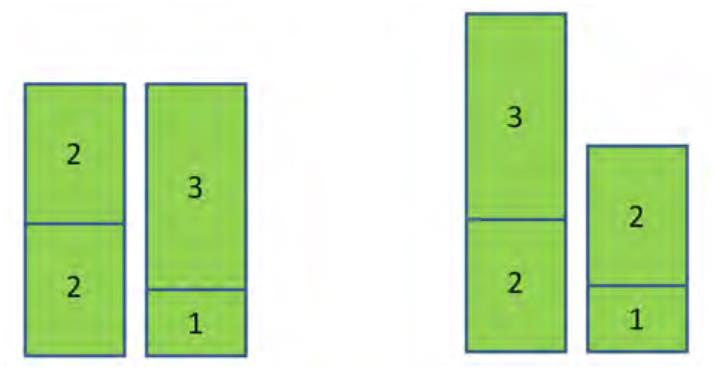


2
.3 Analysis
In the first half of CS261, we were always asking “how do we know when we’re done (i.e.,
optimal)?” This was the appropriate question when the goal was to design an algorithm
that always computes an optimal solution. In an online problem, we don’t expect any online
algorithm to always compute the optimal-in-hindsight solution. We expect to compromise
on the guarantees provided by online algorithms with respect to this benchmark.
In the first half of CS261, we were obsessed with “optimality conditions” — necessary
and sufficient conditions on a feasible solution for it to be an optimal solution. In the second
half of CS261, we’ll be obsessed with bounds on the optimal solution — quantities that are
“only better than optimal.” Then, if our algorithm’s performance is not too far from our
bound, then it is also not too far from the optimal solution.
Where do such bounds come from? For the two case studies today, simple bounds suffice
for our purposes. Next lecture we’ll use LP duality to obtain such bounds — this will
demonstrate that the same tools that we developed to prove the optimality of an algorithm
can also be useful in proving approximate optimality.
The next two lemmas give two different simple lower bounds on the minimum-possible
makespan (call it OPT), given m machines and jobs with processing times p , . . . , p .
1
n
Lemma 2.1 (Lower Bound #1)
n
OPT ≥ max p .
j=1
j
Lemma 2.1 should be clear enough — the biggest job has to go somewhere, and wherever it
is assigned, that machine’s load (and hence the makespan) will be at least as big as the size
of this job.
The second lower bound is almost as simple.
Lemma 2.2 (Lower Bound #2)
Xn
1
OPT ≥
p .
j
m
j=1
Proof: In every schedule, we have
maximum load of a machine ≥ average load of a machine
Xn
1
=
p .
j
m
j=1
ꢀ
These two lemmas imply the following guarantee for Graham’s algorithm.
Theorem 2.3 The makespan of the schedule output by Graham’s algorithm is always at
most twice the minimum-possible makespan (in hindsight).
3


In online algorithms jargon, Theorem 2.3 asserts that Graham’s algorithm is 2-competitive,
or equivalently has a competitive ratio of at most 2.
Theorem 2.3 is tight in the worst case (as m → ∞), though better bounds are possible
in the (often realistic) special case where all jobs are relatively small (see Exercise Set #7).
Proof of Theorem 2.3: Consider the final schedule produced by Graham’s algorithm, and
suppose machine i determines the makespan (i.e., has the largest load). Let j denote the
last job assigned to i. Why was j assigned to i at that point? It must have been that, at
that time, machine i had the smallest load (by the definition of the algorithm). Thus prior
to j’s assignment, we had
load of i = minimum load of a machine (at that time)
≤
average load of a machine (at that time)
Xj−1
1
=
p .
k
m
k=1
Thus,
Xj−1
1
final load of machine i ≤
p + p
k
j
m
|{z}
k=1
{z }
|
≤
OPT
≤
2OP T,
OPT
≤
with the last inequality following from our two lower bounds on OPT (Lemma 2.1 and 2.2).
ꢀ
Theorem 2.3 should be taken as a representative result in a very large literature. Many
good guarantees are known for different online scheduling algorithms and different scheduling
problems.
3
Online Steiner Tree
We have two more case studies in online algorithms: the online Steiner tree problem (this
lecture) and the online bipartite matching problem (next lecture).2
3
.1 Problem Definition
In the online Steiner tree problem:
2
Because the benchmark of the best-possible solution in hindsight is so strong, for many important
problems, all online algorithm have terrible competitive ratios. In these cases, it is important to change the
setup so that theory can still give useful advice about which algorithm to use. See the instructor’s CS264
course (“beyond worst-case analysis”) for much more on this. In CS261, we’ll cherrypick a few problems
where there are natural online algorithms with good competitive ratios.
4


•
•
an algorithm is given in advance a connected undirected graph G = (V, E) with a
nonnegative cost ce ≥ 0 for each edge e ∈ E;
“terminals” t , . . . , t ∈ V arrive online (i.e., one-by-one).
1
k
The requirement for an online algorithm is to maintain at all times a subgraph of G that
spans all of the terminals that have arrived thus far. Thus when a new terminal arrives, the
algorithm must connect it to the subgraph-so-far. Think, for example, of a cable company
as it builds new infrastructure to reach emerging markets. The gold standard is to compute
the minimum-cost subgraph that spans all of the terminals (the “Steiner tree”).3 The goal
of an online algorithm is to get as close as possible to this gold standard.
3
.2 Metric Case vs. General Case
A seemingly special case of the online Steiner tree problem is the metric case. Here, we
assume that:
1
2
. The graph G is the complete graph.4
. The edges satisfy the triangle inequality: for every triple u, v, w ∈ V of vertices,
cuw ≤ c + c .
uv
vw
The triangle inequality asserts that the shortest path between any two vertices is the direct
edge between the vertices (which exists, since G is complete) — that is, adding intermediate
destinations can’t help. The condition states that one-hop paths are always at least as good
as two-hop paths; by induction, one-hop paths are as good as arbitrary paths between the
two endpoints.
For example, distances between points in a normed space (like Euclidean space) satisfy
the triangle inequality. Fares for airline tickets are a non-example: often it’s possible to get
a cheaper price by adding intermediate stops.
It turns out that the metric case of the online Steiner tree problem is no less general than
the general case.
Lemma 3.1 Every α-competitive online algorithm for the metric case of the online Steiner
tree problem can be transformed into an α-competitive online algorithm for the general online
Steiner tree problem.
Exercise Set #7 asks you to supply the proof.
3
4
Since costs are nonnegative, this is a tree, without loss of generality.
By itself, this is not a substantial assumption — one could always complete an arbitrary graph with
super-high-cost edges.
5

3
.3 The Greedy Algorithm
We’ll study arguably the most natural online Steiner tree algorithm, which greedily connects
a new vertex to the subgraph-so-far in the cheapest-possible way.5
Greedy Online Steiner Tree
initialize T ⊆ E to the empty set
for each terminal arrival t , i = 2, . . . , k do
i
add to T the cheapest edge of the form (t , t ) with j < i
i
j
For example, in the 11th iteration of the algorithm, the algorithm looks at the 10 edges
between the new terminal and the terminals that have already arrived, and connects the
new terminal via the cheapest of these edges.6
3
.4 Two Examples
2
t2
1
t1
a
2
1
1
t3
2
Figure 2: First example.
For example, consider the graph in Figure 2, with edge costs as shown. (Note that the
triangle inequality holds.) When the first terminal t1 arrives, the online algorithm doesn’t
have to do anything. When the second terminal t2 arrives, the algorithm adds the edge
(t , t ), which has cost 2. When terminal t arrives, the algorithm is free to connect it to
1
2
3
either t or t (both edges have cost 2). In any case, the greedy algorithm constructs a
1
2
5
What else could you do? An alternative would be to build some extra infrastructure, hedging against
the possibility of future terminals that would otherwise require redundant infrastructure. This idea actually
beats the greedy algorithm in non-worst-case models (see CS264).
6
This is somewhat reminiscent of Prim’s minimum-spanning tree algorithm. The difference is that Prim’s
algorithm processes the vertices in a greedy order (the next vertex to connect is the closest one), while the
greedy algorithm here is online, and has to process the terminals in the order provided.
6

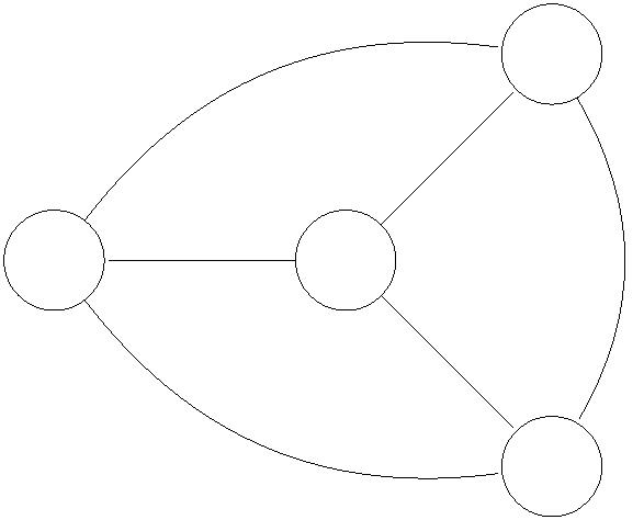

subgraph with total cost 4. Note that the optimal Steiner tree in hindsight has cost 3 (the
spokes).
t1
1
4
2
3
t5
t3
t4
t2
1
1
3
1
2
2
Figure 3: Second example.
For a second example, consider the graph in Figure 3. Again, the edge costs obey the
triangle inequality. When t arrives, the algorithm does nothing. When t arrives, the
1
algorithm adds the edge (t , t ), which has cost 4. When t arrives, there is a tie between
2
1
2
the edges (t , t ) and (t , t ), which both have cost 2. Let’s say that the algorithm picks the
3
1
latter. When terminals t and t arrive, in each case there are two unit-cost options, and it
3
2
3
4
5
doesn’t matter which one the algorithm picks. At the end of the day, the total cost of the
greedy solution is 4 + 2 + 1 + 1 = 8. The optimal solution in hindsight is the path graph
t -t -t -t -t , which has cost 4.
1
5
3
4
2
3
.5 Lower Bounds
The second example above shows that the greedy algorithm cannot be better than 2-
competitive. In fact, it is not constant-competitive for any constant.
Proposition 3.2 The (worst-case) competitive ratio of the greedy online Steiner tree algo-
rithm is Ω(log k), where k is the number of terminals.
Exercise Set #7 asks you to supply the proof, by extending the second example above.
The following result is harder to prove, but true.
Proposition 3.3 The (worst-case) competitive ratio of every online Steiner tree algorithm,
deterministic or randomized, is Ω(log k).
3
.6 Analysis of the Greedy Algorithm
We conclude the lecture with the following result.
7
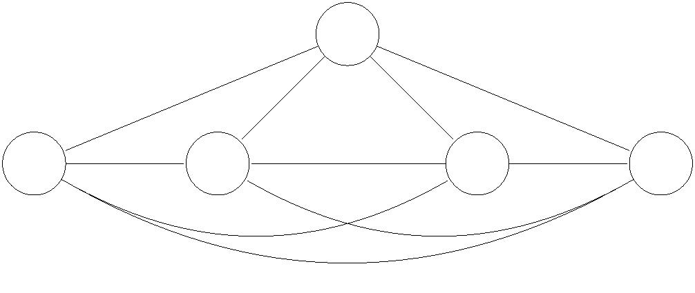
Theorem 3.4 The greedy online Steiner tree algorithm is 2 ln k-competitive, where k is the
number of terminals.
In light of Proposition 3.3, we conclude that the greedy algorithm is an optimal online
algorithm (in the worst case, up to a small constant factor).
The theorem follows easily from the following key lemma, which relates the costs incurred
by the greedy algorithm to that of the optimal solution in hindsight.
Lemma 3.5 For every i = 1, 2, . . . , k − 1, the ith most expensive edge in the greedy solution
T has cost at most 2OP T/i, where OPT is the cost of the optimal Steiner tree in hindsight.
Thus, the most expensive edge in the greedy solution has cost at most 2OPT, the second-
most expensive edge costs at most OPT, the third-most at most 2OP T/3, and so on. Recall
that the greedy algorithm adds exactly one edge in each of the k −1 iterations after the first,
so Lemma 3.5 applies (with a suitable choice of i) to each edge in the greedy solution.
To apply the key lemma, imagine sorting the edges in the final greedy solution from
most to least expensive, and then applying Lemma 3.5 to each (for successive values of
i = 1, 2, . . . , k − 1). This gives
Xk−1
Xk−1
2
OPT
i
1
greedy cost ≤
= 2OPT
≤ (2 ln k) · OP T,
i
i=1
i=1
where the last inequality follows by estimating the sum by an integral.
It remains to prove the key lemma.
Proof of Lemma 3.5: The proof uses two nice tricks, “tree-doubling” and “shortcutting,”
both of which we’ll reuse later when we discuss the Traveling Salesman Problem.
We first recall an easy fact from graph theory. Suppose H is a connected multi-graph (i.e.,
parallel copies of an edge are OK) in which every vertex has even degree (a.k.a. an “Eulerian
graph”). Then H has an Euler tour, meaning a closed walk (i.e., a not-necessarily-simple
cycle) that uses every edge exactly once. See Figure 4. The all-even-degrees condition is
clearly necessary, since if the tour visits a vertex k times then it must have degree 2k. You’ve
probably seen the proof of sufficiency in a discrete math course; we leave it to Exercise Set
#
7.7
t2
t3
t1
t4
Figure 4: Example graph with Euler tour t -t -t -t -t -t .
1
2
3
1
4
1
7
Basically, you just peel off cycles one-by-one until you reach the empty graph.
8


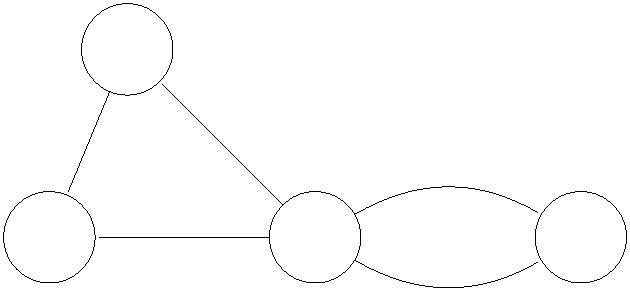

∗
Next, let T be the optimal Steiner tree (in hindsight) spanning all of the terminals
P
∗
c denote its cost. Obtain H from T by adding a second copy
of every edge (Figure 5). Obviously, H is Eulerian (every vertex degree got doubled) and
t , . . . , t . Let OPT =
1
k
∈
∗
e
e
T
P
c = 2OPT. Let C denote an Euler tour of H. C visits each of the terminals at least
e∈H
e
one, perhaps multiple times, and perhaps visits some other vertices as well. Since C uses
P
every edge of H once,
ce = 2OPT.
e∈C
t2
t2
t1
t4
t1
t4
t3
t3
Figure 5: (a) Before doubling edges and (b) after doubling edges.
Now fix a value for the parameter i ∈ {1, 2, . . . , k − 1} in the lemma statement. Define
the “connection cost” of a terminal t with j > 1 as the cost of the edge that was added to
j
the greedy solution when t arrived (from t to some previous terminal). Sort the terminals
j
j
in hindsight in nonincreasing order of connection cost, and let s , . . . , s be the first (most
1
i
expensive) i terminals. The lemma asserts that the cheapest of these has connection cost
at most 2OP T/i. (The ith most expensive terminal is the cheapest of the i most expensive
terminals.)
The tour C visits each of s , . . . , s at least once. “Shortcut” it to obtain a simple cycle C
i
1
i
on the vertex set {s , . . . , s } (Figure 6). For example, if the first occurrences of the terminals
1
in C happen to be in the order s , . . . , s , then C is just the edges (s , s ), (s , s ), . . . , (s , s ).
i
1
i
i
1
2
2
3
i
1
In any case, the order of terminals on Ci is the same as that of their first occurrences in C.
Since the edge costs satisfy the triangle inequality, replacing a path by a direct edge between
P
P
its endpoints can only decrease the cost. Thus
has i edges,
ce ≤
c = 2OPT. Since C only
e
e∈Ci
e
∈
C
i
X
1
min ce
≤
c
≤ 2OP T/i.
e
i
e∈C
|
{z
i
}
e∈C
|
{z
i
}
cheapest edge
average edge cost
Thus some edge (s , s ) ∈ C has cost at most 2OP T/i.
h
j
i
9
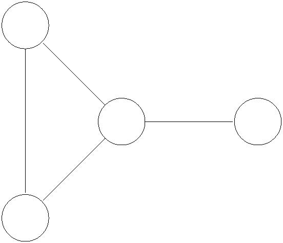
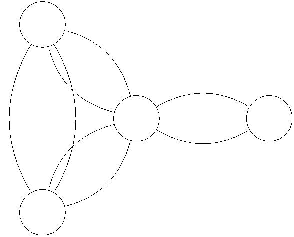


t1
t2
t3
Figure 6: (a) Solid edges represent original edges, and dashed edge represent edges after
shortcutting from t to t , t to t , t to t has been done.
1
2
2
3
3
1
Consider whichever of s , s arrives later in the online ordering, say s . Since s arrived
h
j
j
h
earlier, the edge (s , s ) is one option for connecting s to a previous terminal; the greedy
h
j
j
algorithm either connects sj via this edge or by one that is even cheaper. Thus at least one
vertex of {s , . . . , s }, namely s , has connection cost at most 2OP T/i. Since these are by
1
i
j
definition the terminals with the i largest connection costs, the proof is complete. ꢀ
1
0
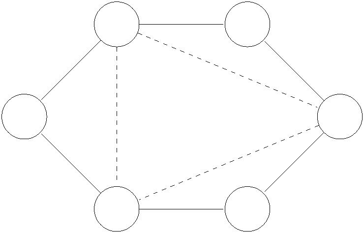
CS261: A Second Course in Algorithms
Lecture #14: Online Bipartite Matching∗
Tim Roughgarden†
February 18, 2016
1
Online Bipartite Matching
Our final lecture on online algorithms concerns the online bipartite matching problem. As
usual, we need to specify how the input arrives, and what decision the algorithm has to make
at each time step. The setup is:
•
•
The left-hand side vertices L are known up front.
The right-hand side vertices R arrive online (i.e., one-by-one). A vertex w ∈ R arrives
together with all of the incident edges (the graph is bipartite, so all of w’s neighbors
are in L).
•
The only time that a new vertex w ∈ R can be matched is immediately on arrival.
The goal is to construct as large a matching as possible. (There are no edge weights, we’re
just talking about maximum-cardinality bipartite matching.) We’d love to just wait until all
of the vertices of R arrive and then compute an optimal matching at the end (e.g., via a max
flow computation). But with the vertices of R arriving online, we can’t expect to always do
as well as the best matching in hindsight.
This lecture presents the ideas behind optimal (in terms of worst-case competitive ratio)
deterministic and randomized online algorithms for online bipartite matching. The random-
ized algorithm is based on a non-obvious greedy algorithm. While the algorithms do not
reference any linear programs, we will nonetheless prove the near-optimality of our algo-
rithms by exhibiting a feasible solution to the dual of the maximum matching problem. This
demonstrates that the tools we developed for proving the optimality of algorithms (for max
flow, linear programming, etc.) are more generally useful for establishing the approximate
optimality of algorithms. We will see many more examples of this in future lectures.
∗
†
ꢀc
2
Department of Computer Science, Stanford University, 474 Gates Building, 353 Serra Mall, Stanford,
016, Tim Roughgarden.
CA 94305. Email: tim@cs.stanford.edu.
1

Online bipartite matching was first studied in 1990 (when online algorithms were first
hot), but a new 21st-century killer application has rekindled interest on the problem over
the past 7-8 years. (Indeed, the main proof we present was only discovered in 2013!)
The killer application is Web advertising. The vertices of L, which are known up front,
represent advertisers who have purchased a contract for having their ad shown to users that
meet specified demographic criteria. For example, an advertiser might pay (in advance) to
have their ad shown to women between the ages of 25 and 35 who live within 100 miles of
New York City. If an advertiser purchased 5000 views, then there will be 5000 corresponding
vertices on the left-hand side. The right-hand side vertices, which arrive online, correspond
to “eyeballs.” When someone types in a search query or accesses a content page (a new
opportunity to show ads), it corresponds to the arrival of a vertex w ∈ R. The edges incident
to w correspond to the advertisers for whom w meets their targeting criteria. Adding an
edge to the matching then corresponds to showing a given ad to the newly arriving eyeball.
Both Google and Microsoft (and probably other companies) employ multiple people whose
primary job is adapting and fine-tuning the algorithms discussed in this lecture to generate
as much as revenue as possible.
2
Deterministic Algorithms
v1
w1
v2
w2
1
Figure 1: Graph where no deterministic algorithm has competitive ratio better than .
2
1
We first observe that no deterministic algorithm has a competitive ratio better than .
Consider the example in Figure 1. The two vertices v , v on the left are known up front,
2
1
2
and the first vertex w1 to arrive on the right is connected to both. Every deterministic
algorithm picks either the edge (v , w ) or (v , w ).1 In the former case, suppose the second
1
vertex w to arrive is connected only to v , which is already matched. In this case the online
1
2
1
2
algorithm’s solution has 1 edge, while the best matching in hindsight has size 2. The other
1
case is symmetric. Thus for every deterministic algorithm, there is an instance where the
1
matching it outputs is at most times the maximum possible in hindsight.
2
1
Technically, the algorithm could pick neither, but then its competitive ratio would be 0 (what if no more
vertices arrive?).
2
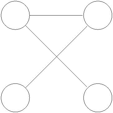


1
The obvious greedy algorithm has a matching competitive ratio of . By the “obvious
2
algorithm” we mean: when a new vertex w ∈ R arrives, match w to an arbitrary unmatched
neighbor (or to no one, if it has no unmatched neighbors).
1
Proposition 2.1 The deterministic greedy algorithm has a competitive ratio of .
2
Proof: The proposition is easy to prove directly, but here we’ll give a more-sophisticated-
than-necessary proof because it introduces ideas that we’ll build on in the randomized case.
Our proof uses a dual feasible solution as an upper bound on the size of a maximum matching.
Recall the relevant primal-dual pair ((P) and (D), respectively):
X
max
xe
e∈E
subject to
X
xe ≤ 1
for all v ∈ L ∪ R
for all e ∈ E,
e∈δ(v)
xe ≥ 0
min
and
X
pv
v∈L∪R
subject to
p + p ≥ 1
for all (v, w) ∈ E
for all v ∈ L ∪ R.
v
w
p ≥ 0
v
There are some minor differences with the primal-dual pair that we considered in Lecture
9, when we discussed the minimum-cost perfect matching problem. First, in (P), we’re
#
maximizing cardinality rather than minimizing cost. Second, we allow matchings that are
not perfect, so the constraints in (P) are inequalities rather than equalities. This leads to the
expected modifications of the dual: it is a minimization problem rather than a maximization
problem, therefore with greater-than-or-equal-to constraints rather than less-than-or-equal-
to constraints. Because the constraints in the primal are now inequality constraints, the dual
variables are now nonnegative (rather than unrestricted).
We use these linear programs (specifically, the dual) only for the analysis; the algorithm,
remember, is just the obvious greedy algorithm. We next define a “pre-dual solution” as
follows: for every v ∈ L ∪ R, set
ꢀ
1
2
0
if greedy matches v
otherwise.
qv =
The q’s are defined in hindsight, purely for the sake of analysis. Or if you prefer, we can
imagine initializing all of the qv’s to 0 and then updating them in tandem with the execution
3

of the greedy algorithm — when the algorithm adds a vertex (v, w) to its matching, we set
1
both q and q to . (Since the chosen edges form a matching, a vertex has its q-value set
1
v
to at most once.) This alternative description makes it clear that
w
2
2
X
|
M| =
q ,
v
(1)
v∈L∪R
where M is the matching output by the greedy algorithm. (Whenever one edge is added to
1
the matching, two vertices have their q-values increased to .)
2
Next, observe that for every edge (v, w) of the final graph (L∪R, E), at least one of q , q
v
is (if not both). For if q = 0, then v was not matched by the algorithm, which means that
w
1
2
v
w had at least one unmatched neighbor when it arrived, which means the greedy algorithm
1
matched it (presumably to some other unmatched neighbor) and hence q = .
w
2
This observation does not imply that q is a feasible solution to the dual linear pro-
gram (D), which requires a sum of at least 1 from the endpoints of every edge. But it does
imply that after scaling up q by a factor 2 to obtain p = 2q, p is feasible for (D). Thus
X
1
2
1
|
M| =
pv ≥ · OP T,
{z }
2
v∈L∪R
|
obj fn of p
where OPT denotes the size of the maximum matching in hindsight. The first equation is
from (1) and the definition of p, and the inequality is from weak duality (when the primal
is a maximization problem, every feasible dual solution provides an upper bound on the
optimum). ꢀ
3
Online Fractional Bipartite Matching
3
.1 The Problem
We won’t actually discuss randomized algorithms in this lecture. Instead, we’ll discuss a
deterministic algorithm for the fractional bipartite matching problem. The keen reader will
object that this is a stupid idea, because we’ve already seen that the fractional and integral
bipartite matching problems are really the same.2 While it’s true that fractions don’t help
the optimal solution, they do help an online algorithm, intuitively by allowing it to “hedge.”
This is already evident in our simple bad example for deterministic algorithms (Figure 1).
When w1 shows up, in the integral case, a deterministic online algorithm has to match w1
fully to either v or v . But in the fractional case, it can match w 50/50 to both v and
1
2
1
1
v . Then when w arrives, with only one neighbor on the left-hand side, it can at least be
1
2
matched with a fractional value of . The online algorithm produces a fractional matching
2
2
2
In Lecture #9 we used the correctness of the Hungarian algorithm to argue that the fractional problem
always has a 0-1 optimal solution (since the algorithm terminates with an integral solution and a dual-feasible
solution with same objective function value). See also Exercise Set #5 for a direct proof of this.
4


3
2
3
4
with value while the optimal solution has size 2. So this only proves a bound of of
the best-possible competitive ratio, leaving open the possibility of online algorithms with
1
competitive ratio bigger than .
2
3
.2 The Water Level (WL) Algorithm
We consider the following “Water Level,” algorithm, which is a natural way to define “hedg-
ing” in general.
Water-Level (WL) Algorithm
Physical metaphor:
think of each vertex v ∈ L as a water container with a capacity of 1
think of each vertex w ∈ R as a source of one unit of water
when w ∈ R arrives:
drain water from w to its neighbors, always preferring the containers
with the lowest current water level, until either
(i) all neighbors of w are full; or
(ii) w is empty (i.e., has sent all its water)
See also Figure 2 for a cartoon of the water being transferred to the neighbors of a vertex
w. Initially the second neighbor has the lowest level so w only sends water to it; when the
water level reaches that of the next-lowest (the fifth neighbor), w routes water at an equal
rate to both the second and fifth neighbors; when their common level reaches that of the
third neighbor, w routes water at an equal rate to these three neighbors with the lowest
current water level. In this cartoon, the vertex w successfully transfers its entire unit of
water (case (ii)).
Figure 2: Cartoon of water being transferred to vertices.
5


For example, in the example in Figure 1, the WL algorithm replicates our earlier hedging,
with vertex w distributing its water equally between v and v (triggering case (ii)) and
1
1
2
1
vertex w2 distributing units of water to its unique neighbor (triggering case (i)).
2
This algorithm is natural enough, but all you’ll have to remember for the analysis is the
following key property.
Lemma 3.1 (Key Property of the WL Algorithm) Let (v, w) ∈ E be an edge of the
P
final graph G and y =
x the final water level of the vertex v ∈ L. Then w only sent
v
water to containers when their current water level was y or less.
∈
e
e
δ(v)
v
Proof: Fix an edge (v, w) with v ∈ L and w ∈ R. The lemma is trivial if y = 1, so suppose
v
y < 1 — that the container v is not full at the end of the WL algorithm. This means
v
that case (i) did not get triggered, so case (ii) was triggered, so the vertex w successfully
routed all of its water to its neighbors. At the time when this transfer was completed, all
containers to which w sent some water have a common level `, and all other neighbors of w
have current water level at least ` (cf., Figure 2). At the end of the algorithm, since water
levels only increase, all neighbors of w have final water level ` or more. Since w only sent
flow to containers when their current water level was ` or less, the proof is complete. ꢀ
3
.3 Analysis: A False Start
To prove a bound on the competitive ratio of the WL algorithm, a natural idea is to copy
the same analysis approach that worked so well for the integral case (Proposition 2.1). That
is, we define a pre-dual solution in tandem with the execution of the WL algorithm, and
then scale it up to get a solution feasible for the dual linear program (D) in Section 2.
Idea #1:
•
•
initialize qv = 0 for all v ∈ L ∪ R;
whenever the amount xvw of water sent from w to v goes up by ∆, increase both qv
and qw by ∆/2.
Inductively, this process maintains at all times that the value of the current fractional match-
P
ing equals
increases by the same amount.)
The hope is that, for some constant c > , the scaled-up vector p = q is feasible for (D).
If this is the case, then we have proved that the competitive ratio of the WL algorithm is at
qv. (Whenever the matching size increases by ∆, the sum of q-values
v∈L∪R
1
1
2
c
P
least c (since its solution value equals c times the objective function value
pv of the
v∈L∪R
dual feasible solution p, which in turn is an upper bound on the optimal matching size).
To see why this doesn’t work, consider the example shown in Figure 3. Initially there
are four vertices on the left-hand side. The first vertex w ∈ R is connected to every vertex
1
of L, so the WL algorithm routes one unit of water evenly across the four edges. Now every
1
4
∈
container has a water level of . The second vertex w
all neighbors have the same water level, w splits its unit of water evenly between the three
R is connected to v , v , v . Since
2
2
3
4
2
6

1
1
3
7
12
∈
containers, bringing their water levels up to + = . The third vertex w3 R is connected
4
only to v and v . The vertex splits its water evenly between these two containers, but it
3
cannot transfer all of its water; after sending
4
5
2
units to each of v and v , both containers
3
4
1
are full (triggering case (i)). The last vertex w ∈ R is connected only to v . Since v is
4
4
4
already full, w can’t get rid of any of its water.
4
The question now is: by what factor to we have to scale up q to get a feasible solution
1
p = q to (D)? Recall that dual feasibility boils down to the sum of p-values of the endpoints
of every edge being at least 1. We can spot the problem by examining the edge (v , w ).
c
4
4
1
2
The vertex v4 got filled, so its final q-value is (as high as it could be with the current
approach). The vertex w4 didn’t participate in the fractional matching at all, so its q-value
1
is 0. Since q + q = , we would need to scale up by 2 to achieve dual feasibility. This
4
v
does not improve over the competitive ration of .
w4
2
1
2
1
/4
1
w1
v1
v2
v3
v4
/4
/4
/4
1
w2
1
/3
1
1
/3
/3
1
5
/12
w3
5
/12
Figure 3: Example showcasing why Idea #1 does not work.
On the other hand, the solution computed by the WL algorithm for this example, while
17
5
not optimal, is also not that bad. Its value is 1 + 1 + + 0 = , which is substantially
1
6
bigger than times the optimal solution (which is 4). Thus this is a bad example only for
6
2
the analysis approach, and not for the WL algorithm itself. Can we keep the algorithm the
same, and just be smarter with its analysis?
7


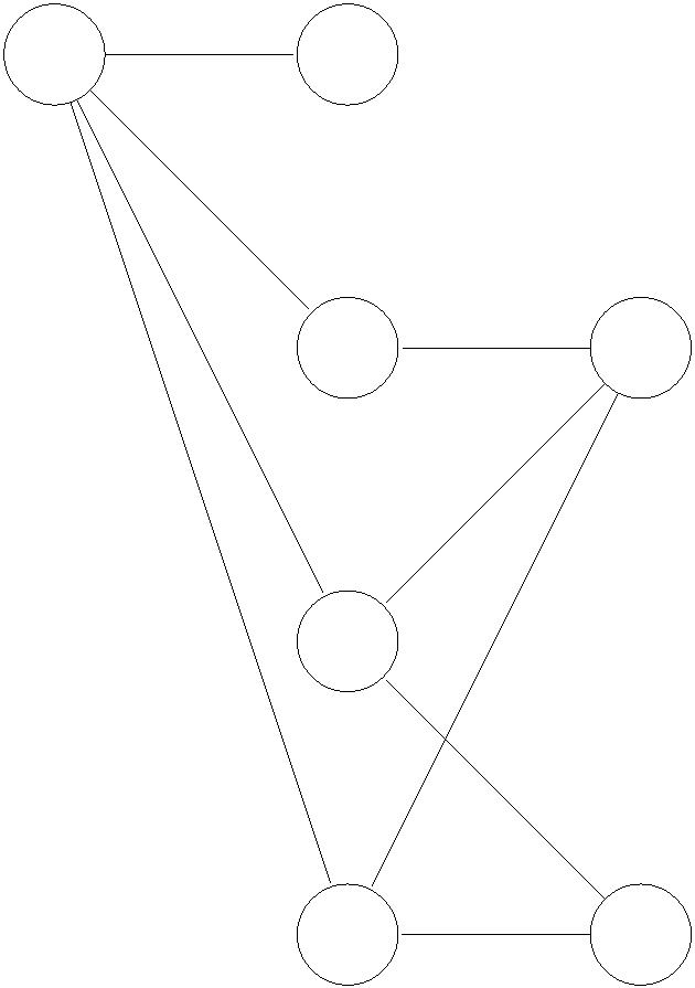
3
.4 Analysis: The Main Idea
Idea #2: when the amount xvw of water sent from w to v goes up by ∆, split the increase
unequally between q and q .
v
To see the motivation for this idea, consider the bottom edge in Figure 3. The WL
w
algorithm never sends any water on any edge incident to w4, so it’s hard to imagine how
1
its q-value will wind up anything other than 0. So if we want to beat , we need to make
1
2
sure that v finishes with a q-value bigger than . A naive fix for this example would be to
4
only increase the q-values for vertices of L, and not from R; but this would fail miserably
2
1
if w were the only vertex to arrive (then all q-values on the left would be , all those on
1
4
the right 0). To hedge between the various possibilities, as a vertex v ∈ L gets more and
more full, we will increase its q-value more and more quickly. Provided it increases quickly
enough as v becomes full, it is conceivable that v could end up with a q-value bigger than
1
2
.
with the splitting ratio evolving over the course of the algorithm.
Summarizing, we’ll use unequal splits between the q-values of the endpoints of an edge,
There are zillions of ways to split an increase of ∆ on xvw between q and q (as a function
v
w
of v’s current water level). The plan is to give a general analysis that is parameterized by such
a “splitting function,” and solve for the splitting function that leads to the best competitive
ratio. Don’t forget that all of this is purely for the analysis; the algorithm is always the WL
algorithm.
So fix a nondecreasing “splitting function” g : [0, 1] → [0, 1]. Then:
•
•
initialize qv = 0 for all v ∈ L ∪ R;
whenever the amount xvw of water sent from w to v goes up by an infinitesimal amount
dz, and the current water level of v is yv =
P
x :
δ(v)
∈
e
e
–
–
increase q by g(y )dz;
v
v
increase q by (1 − g(y ))dz.
w
v
For example, if g is the constant function always equal to 0 (respectively, 1), then only
the vertices of R (respectively, vertices of L) receive positive q-values. If g is the constant
1
function always equal to , then we recover our initial analysis attempt, with the increase
on an edge split equally between its endpoints.
By construction, no matter how we choose the function g, we have
2
X
current value of WL fractional matching = current value of
q ,
v
v∈L∪R
at all times, and in particular at the conclusion of the algorithm.
For the analysis (parameterized by the choice of g), fix an arbitrary edge (v, w) of the
1
2
final graph. We want a worst-case lower bound on q + q (hopefully, bigger than ).
v
w
8

For the first case, suppose that at the termination of the WL algorithm, the vertex v ∈ L
P
is full (i.e., y =
x = 1). At the time that v’s current water level was z, it accrued
δ(v)
v
q-value at rate g(z). Integrating over these accruals, we have
∈
e
e
Z
1
q + q ≥ q =
g(z)dz.
(2)
v
w
v
0
(It may seem sloppy to throw out the contribution of q ≥ 0, but Figure 3 shows that when
w
v is full it might well be the case that some of its neighbors have q-value 0.) Note that the
bigger the function g is, the bigger the lower bound in (2).
For the second case, suppose that v only has water level yv < 1 at the conclusion of the
WL algorithm. It follows that w successfully routed its entire unit of water to its neighbors
(otherwise, the WL algorithm would have routed more water to the non-full container v).
Here’s where we use the key property of the WL algorithm (Lemma 3.1): whenever v sent
water to a container, the current water level of that container was as most yv. Thus, since
the function g is nondecreasing, whenever v routed any water, it accrued q-value at rate at
least 1 − g(yv). Integrating over the unit of water sent, we obtain
Z
1
qw ≥
(1 − g(y ))dz = 1 − g(y ).
v
v
0
As in the first case, we have
and hence
Z
yv
qv =
g(z)dz
0
ꢁ
Z
ꢂ
yv
q + q ≥
g(z)dz + 1 − g(y ).
(3)
v
w
v
0
Note the lower bound in (3) is generally larger for smaller functions g (since 1 − g(y ) is
v
bigger). This is the tension between the two cases.
For example, if we take g to be identically 0, then the lower bounds (2) and (3) read 0
and 1, respectively. With g identically equal to 1, the values are reversed. With g identically
1
equal to , as in our initial attempt, the right-hand sides of both (2) and (3) are guaranteed
1
2
to be at least (though not larger).
2
3
.5 Solving for the Optimal Splitting Function
With our lower bounds (2) and (3) on the worst-case value of q + q for an edge (v, w), our
v
w
task is clear: we want to solve for the splitting function g that makes the minimum of these
two lower bounds as large as possible. If we can find a function g such that the right-hand
sides of (2) and (3) (for any y ∈ [0, 1]) are both at least c, then we will have proved that
v
the WL algorithm is c-competitive. (Recall the argument: the value of the WL matching is
P
1
c
q , and p = q is a feasible dual solution, which is an upper bound on the maximum
v
matching.)
v
9

Solving for the best nondecreasing splitting function g may seem an intimidating prospect
there are an infinite number of functions to choose from. In situations like this, a good
—
strategy is to “guess and check” — try to develop intuition for what the right answer might
look like and then verify your guess. There are many ways to guess, but often in an optimal
analysis there is “no slack anywhere” (since otherwise, a better solution could take advantage
of this slack). In our context, this corresponds to guessing that the optimal function g
equalizes the lower bound in (2) with that in (3), and with the second lower bound tight
simultaneously for all values of y ∈ [0, 1]. There is no a priori guarantee that such a g exists,
v
and if such a g exists, its optimality still needs to be verified. But it’s still a good strategy
for generating a guess.
Let’s start with the guess that the lower bound in (3) is the same for all values of
yv ∈ [0, 1]. This means that
ꢁZ
when viewed as a function of y , is a constant function. This means its derivative (w.r.t. y )
ꢂ
yv
g(z)dz + 1 − g(y ),
v
0
v
v
is 0, so
0
g(y ) − g (y ) = 0,
v
v
i.e., the derivative of g is the same as g.3 This implies that g(z) has the form g(z) = kez for
a constant k > 0. This is great progress: instead of an infinite-dimensional g to solve for,
we now just have the single parameter k to solve for.
Now let’s use the guess that the two lower bounds in (2) and (3) are the same. Plugging
kez into the lower bound in (2) gives
Z
1
z
z 1
0
ke dz = k [e | = k(e − 1),
0
which gets larger with k. Plugging kez into the lower bound in (3) gives (for any y ∈ [0, 1])
Z
This lower bound is independent of the choice of y — we knew that would happen, it’s how
z
y
y
y
ke dz + 1 − ke = k(e − 1) + 1 − ke = 1 − k.
0
we chose g(z) = kez – and gets larger with smaller k. Equalizing the two lower bounds of
k(e−1) and 1−k and solving for k, we get k = , and so the splitting function is g(y) = ey−1.
1
e
(Thus when a vertex v ∈ L is empty it gets a share of the increase of an incident edge;
1
e
the share increases as v gets more full, and approaches 100% as v becomes completely full.)
Our lower bounds in (2) and (3) are then both equal to
1
1
−
≈ 63.2%.
e
This proves that the WL algorithm is (1 − )-competitive, a significant improvement over
1
e
1
2
the more obvious -competitive algorithm.
3
I don’t know about you, but this is pretty much the only differential equation that I remember how to
solve.
1
0


3
.6 Epilogue
In this lecture we gave a (1 − )-competitive (deterministic) online algorithm for the online
1
e
fractional bipartite matching problem. The same ideas can be used to design a randomized
online algorithm for the original integral online bipartite matching problem that always
outputs a matching with expected size at least 1 − times the maximum possible. (The
1
e
expectation is over the random coin flips made by the algorithm.) The rough idea is to set
things up so that the probability that a given edge is included the matching plays the same
role as its fractional value in the WL algorithm. Implementing this idea is not trivial, and
the details are outlined in Problem Set #4.
But can we do better? Either with a smarter algorithm, or with a smarter analysis
of these same algorithms? (Recall that being smarter improved the analysis of the WL
1
2
− 1
− 1
algorithm from a to a 1
is negative: no online algorithm, deterministic or randomized, has a competitive ratio better
.) Even though 1
may seem like a weird number, the answer
e
e
than 1 − for maximum bipartite matching. The details of this argument are outlined in
1
e
Problem Set #3.
1
1

CS261: A Second Course in Algorithms
Lecture #15: Introduction to Approximation
Algorithms∗
Tim Roughgarden†
February 23, 2016
1
Coping with NP-Completeness
All of CS161 and the first half of CS261 focus on problems that can be solved in polynomial
time. A sad fact is that many practically important and frequently occurring problems do
not seem to be polynomial-time solvable, that is, are NP-hard.1
As an algorithm designer, what does it mean if a problem is NP-hard? After all, a
real-world problem doesn’t just go away after you realize that it’s NP-hard. The good news
is that NP-hardness is not a death sentence — it doesn’t mean that you can’t do anything
practically useful. But NP-hardness does throw the gauntlet to the algorithm designer, and
suggests that compromises may be necessary. Generally, more effort (computational and
human) will lead to better solutions to NP-hard problems. The right effort vs. solution
quality trade-off depends on the context, as well as the relevant problem size. We’ll discuss
algorithmic techniques across the spectrum — from low-effort decent-quality approaches to
high-effort high-quality approaches.
So what are some possible compromises? First, you can restrict attention to a relevant
special case of an NP-hard problem. In some cases, the special case will be polynomial-
time solvable. (Example: the Vertex Cover problem is NP-hard in general graphs, but on
Problem Set #2 you proved that, in bipartite graphs, the problem reduces to max flow/min
cut.) In other cases, the special case remains NP-hard but is still easier than the general
case. (Example: the Traveling Salesman Problem in Lecture #16.) Note that this approach
requires non-trivial human effort — implementing it requires understanding and articulating
∗
†
ꢀc
2
Department of Computer Science, Stanford University, 474 Gates Building, 353 Serra Mall, Stanford,
016, Tim Roughgarden.
CA 94305. Email: tim@cs.stanford.edu.
I will assume that you’re familiar with the basics of NP-completeness from your other courses, like
CS154. If you want a refresher, see the videos on the Course site.
1
1

whatever special structure your particular application has, and then figuring out how to
exploit it algorithmically.
A second compromise is to spend more than a polynomial amount of time solving the
problem, presumably using tons of hardware and/or restricting to relatively modest problem
sizes. Hopefully, it is still possible to achieve a running time that is faster than naive brute-
force search. While NP-completeness is sometimes interpreted as “there’s probably nothing
better than brute-force search,” the real story is more nuanced. Many NP-complete problems
can be solved with algorithms that, while running in exponential time, are significantly faster
than brute-force search. Examples that we’ll discuss later include 3SAT (with a running
time of (4/3)n rather than 2n) and the Traveling Salesman Problem (with a running time
of 2n instead of n!). Even for NP-hard problems where we don’t know any algorithms that
provably beat brute-force search in the worst case, there are almost always speed-up tricks
that help a lot in practice. These tricks tend to be highly dependent on the particular
application, so we won’t really talk about any in CS261 (where the focus is on general
techniques).
A third compromise, and the one that will occupy most of the rest of the course, is to
relax correctness. For an optimization problem, this means settling for a feasible solution
that is only approximately optimal. Of course one would like the approximation to be as
good as possible. Algorithms that are guaranteed to run in polynomial time and also be
near-optimal are called approximation algorithms, and they are the subject of this and the
next several lectures.
2
Approximation Algorithms
In approximation algorithm design, the hard constraint is that the designed algorithm should
run in polynomial time on every input. For an NP-hard problem, assuming P = NP, this
necessarily implies that the algorithm will compute a suboptimal solution in some cases.
The obvious goal is then to get as close to an optimal solution as possible (ideally, on every
input).
There is a massive literature on approximation algorithms — a good chunk of the algo-
rithms research community has been obsessed with them for the past 25+ years. As a result,
many interesting design techniques have been developed. We’ll only scratch the surface in
our lectures, and will focus on the most broadly useful ideas and problems.
One take-away from our study of approximation algorithms is that the entire algorithmic
toolbox that you’ve developed during CS161 and CS261 remains useful for the design and
analysis of approximation algorithms. For example, greedy algorithms, divide and conquer,
dynamic programming, and linear programming all have multiple killer applications in ap-
proximation algorithms (we’ll see a few). And there are other techniques, like local search,
which usually don’t yield exact algorithms (even for polynomial-time solvable problems) but
seem particularly well suited for designing good heuristics.
The rest of this lecture sets the stage with four relatively simple approximation algorithms
for fundamental NP-hard optimization problems.
2
2
.1 Example: Minimum-Makespan Scheduling
We’ve already seen a couple of examples of approximation algorithms in CS261. For example,
recall the problem of minimum-makespan scheduling, which we studied in Lecture #13.
There are m identical machines, and n jobs with processing times p , . . . , p . The goal is to
1
n
schedule all of the jobs to minimize the makespan (the maximum load, where the load of a
machine is the sum of the processing times of the jobs assigned to it) — to balance the loads
of the machines as evenly as possible.
In Lecture #13, we studied the online version of this problem, with jobs arriving one-
by-one. But it’s easy to imagine applications where you get to schedule a batch of jobs all
at once. This is the offline version of the problem, with all n jobs known up front. This
problem is NP-hard.2
Recall Graham’s algorithm, which processes the jobs in the given (arbitrary) order, al-
ways scheduling the next job on the machine that currently has the lightest load. This
algorithm can certainly by implemented in polynomial time, so we can reuse it as a legiti-
mate approximation algorithm for the offline problem. (Now the fact that it processes the
jobs online is just a bonus.) Because it always produces a schedule with makespan at most
twice the minimum possible (as we proved in Lecture #13), it is a 2-approximation algo-
rithm. The factor “2” here is called the approximation ratio of the algorithm, and it plays
the same role as the competitive ratio in online algorithms.
Can we do better? We can, by exploiting the fact that an (offline) algorithm knows all of
the jobs up front. A simple thing that an offline algorithm can do that an online algorithm
cannot is sort the jobs in a favorable order. Just running Graham’s algorithm on the jobs
4
in order from largest to smallest already improves the approximation ratio to (a good
homework problem).
3
2
.2 Example: Knapsack
Another example that you might have seen in CS161 (depending on who you took it from)
is the Knapsack problem. We’ll just give an executive summary; if you haven’t seen this
material before, refer to the videos posted on the course site.
An instance of the Knapsack problem is n items, each with a value and a weight. Also
given is a capacity W. The goal is to identify the subset of items with the maximum total
value, subject to having total weight at most W. The problem gets its name from a silly
story of a burglar trying to fill up a sack with the most valuable items. But the problem
comes up all the time, either directly or as a subroutine in a more complicated problem —
whenever you have a shared resource with a hard capacity, you have a knapsack problem.
Students usually first encounter the Knapsack problem as a killer application of dynamic
programming. For example, one such algorithm, which works as long as all item weights
2
For the most part, we won’t bother to prove any NP-hardness results in CS261. The NP-hardness
proofs are all of the exact form that you studied in a course like CS154 — one just exhibits a polynomial-
time reduction from a known NP-hard problem to the current problem. Many of the problems that we
study were among the first batch of NP-complete problems identified by Karp in 1972.
3


are integers, runs in time O(nW). Note that this is not a polynomial-time algorithm, since
the input size (the number of keystrokes needed to type in the input) is only O(n log W).
(Writing down the number W only takes log W digits.) And in fact, the knapsack problem
is NP-hard, so we don’t expect there to be a polynomial-time algorithm. Thus the O(nW)
dynamic programming solution is an example of an algorithm for an NP-hard problem that
beats brute-force search (unless W is exponential in n), while still running in time exponential
in the input size.
What if we want a truly polynomial-time algorithm? NP-hardness says that we’ll have
to settle for an approximation. A natural greedy algorithm, which processes the items in
1
order of value divided by size (“bang-per-buck”) achieves a -approximation, that is, is
guaranteed to output a feasible solution with total value at least 50% times the maximum
2
possible.3 If you’re willing to work harder, then by rounding the data (basically throwing out
the lower-order bits) and then using dynamic programming (on an instance with relatively
small numbers), one obtains a (1 − ꢀ)-approximation, for a user-specified parameter ꢀ > 0,
1
in time polynomial in n and . (By NP-hardness, we expect the running time to blow up
as ꢀ gets close to 0.) This is pretty much the best-case scenario for an NP-hard problem —
arbitrarily close approximation in polynomial time.
ꢀ
2
.3 Example: Steiner Tree
Next we revisit the other problem that we studied in Lecture #13, the Steiner tree problem.
Recall that the input is an undirected graph G = (V, E) with a nonnegative cost c ≥ 0 for
e
each edge e ∈ E. Recall also that there is no loss of generality in assuming that G is the
complete graph and that the edge costs satisfy the triangle inequality (i.e., c ≤ c + c
uw
uv
vw
for all u, v, w ∈ V ); see Exercise Set #7. Finally, there is a set R = {t , . . . , t } of vertices
1
k
called “terminals.” The goal is to compute the minimum-cost subgraph that spans all of the
terminals. We previously studied this problem with the terminals arriving online, but the
offline version of the problem, with all terminals known up front, also makes perfect sense.
In Lecture #13 we studied the natural greedy algorithm for the online Steiner tree prob-
lem, where the next terminal is connected via a direct edge to a previously arriving terminal
in the cheapest-possible way. We proved that the algorithm always computes a Steiner tree
with cost at most 2 ln k times the best-possible solution in hindsight. Since the algorithm is
easy to implement in polynomial time, we can equally well regard it as a 2 ln k-approximation
algorithm (with the fact that it processes terminals online just a bonus). Can we do some-
thing smarter if we know all the terminals up front?
As with job scheduling, better bounds are possible in the offline model because of the
ability to sort the terminals in a favorable order. Probably the most natural order in which
to process the terminals is to always process next the terminal that is the cheapest to connect
to a previous terminal. If you think about it a minute, you realize that this is equivalent to
running Prim’s MST algorithm on the subgraph induced by the terminals. This motivates:
3
Technically, to achieve this for every input, the algorithm takes the better of this greedy solution and
the maximum-value item.
4


The MST heuristic for metric Steiner tree: output the minimum spanning tree of
the subgraph induced by the terminals.
Since the Steiner tree problem is NP-hard and the MST can be computed in polynomial
time, we expect this heuristic to produce a suboptimal solution in some cases. A concrete
example is shown in Figure 1, where the MST of {t , t , t } costs 4 while the optimal Steiner
1
2
3
tree has cost 3. (Thus the cost can be decreased by spanning additional vertices; this is what
makes the Steiner tree problem hard.) Using larger “wheel” graphs of the same type, it can
be shown that the MST heuristic can be off by a factor arbitrarily close to 2 (Exercise Set
#
8). It turns out that there are no worse examples.
2
t2
1
t1
a
2
1
1
t3
2
Figure 1: MST heuristic will pick {t , t }, {t , t } but best Steiner tree (dashed edges) is
1
2
2
3
{
a, t }, {a, t }, {a, t }.
1
2
3
Theorem 2.1 In the metric Steiner tree problem, the cost of the minimum spanning tree of
the terminals is always at most twice the cost of an optimal solution.
Proof: The proof is similar to our analysis of the online Steiner tree problem (Lecture #13),
only easier. It’s easier to relate the cost of the MST heuristic to that of an optimal solution
than for the online greedy algorithm — the comparison can be done in one shot, rather then
on an edge-by-edge basis.
∗
For the analysis, let T denote a minimum-cost Steiner tree. Obtain H from T by adding
a second copy of every edge (Figure 2(a)). Obviously, H is Eulerian (every vertex degree got
∗
P
doubled) and
walk using every edge of H exactly once. We again have
c = 2OPT. Let C denote an Euler tour of H — a (non-simple) closed
e
e∈H
P
ce = 2OPT.
e∈C
b
The tour C visits each of t , . . . , t at least once. “Shortcut” it to obtain a simple cycle C
1
k
on the vertex set {t , . . . , t } (Figure 2(b)); since the edge costs satisfy the triangle inequality,
1
k
b
this only decreases the cost. C minus an edge is a spanning tree of the subgraph induced by
R that has cost at most 2OPT; the MST can only be better. ꢀ
5
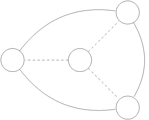
2
t2
2
t2
1
1
1
1
t1
a
2
t1
a
2
1
1
t3
t3
2
2
Figure 2: (a) Adding second copy of each edge in T∗ to form H. Note H is Euler-
sian. (b) Shorting cutting edges ({t1, a}, {a, t2}), ({t2, a}, {a, t3}), ({t3, a}, {a, t1}) to
{
t1, t2}, {t2, t3}, {t3, t1} respectively.
2
.4 Example: Set Coverage
Next we study a problem that we haven’t seen before, set coverage. This problem is a
killer application for greedy algorithms in approximation algorithm design. The input is a
collection S , . . . , S of subsets of some ground set U (each subset described by a list of its
1
m
elements), and a budget k. The goal is to pick k subsets to maximize the size of their union
(Figure 3). All else being equal, bigger sets are better for the set coverage problem. But
it’s not so simple — some sets are largely redundant, while others are uniquely useful (cf.,
Figure 3).
Figure 3: Example set coverage problem. If k = 2, we should pick the blue sets. Although
the red set is the largest, picking it is redundant.
Set coverage is a basic problem that comes up all the time (often not even disguised). For
example, suppose your start-up only has the budget to hire k new people. Each applicant
can be thought of as a set of skills. The problem of hiring to maximize the number of distinct
6
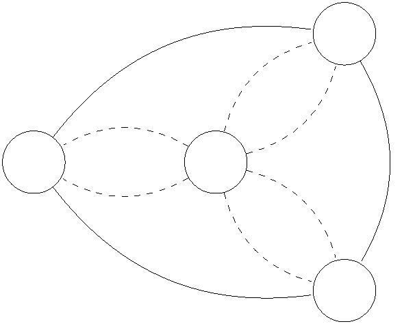
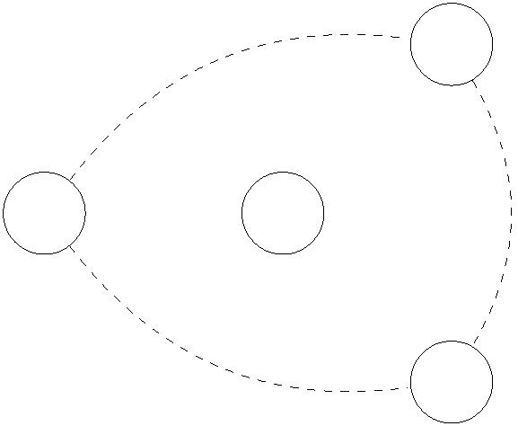
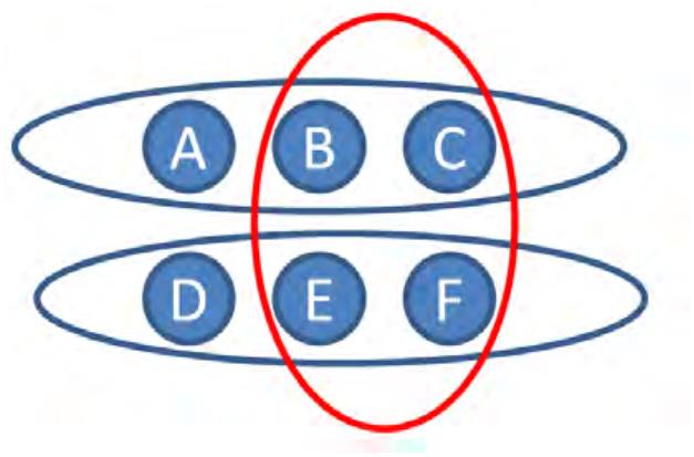
skills required is a set coverage problem. Similarly for choosing locations for factories/fire
engines/Web caches/artisinal chocolate shops to cover as many neighborhoods as possible.
Or, in machine learning, picking a small number of features to explain as much as the data
as possible. Or, in HCI, given a budget on the number of articles/windows/menus/etc. that
can be displayed at any given time, maximizing the coverage of topics/functionality/etc.
The set coverage problem is NP-hard. Turning to approximation algorithms, the follow-
ing greedy algorithm, which increases the union size as much as possible at each iteration,
seems like a natural and good idea.
Greedy Algorithm for Set Coverage
for i = 1, 2, . . . , k: do
compute the set Ai maximizing the number of new elements covered
i−1
(relative to ∪ Aj)
j=1
return {A , . . . , A }
1
k
This algorithm can clearly be implemented in polynomial time, so we don’t expect it to
always compute an optimal solution. It’s useful to see some concrete examples of what can
go wrong. example.
Figure 4: (a) Bad example when k = 2 (b) Bad example when k = 3.
For the first example (Figure 4(a)), set the budget k = 2. There are three subsets. S1
and S partition the ground set U half-half, so the optimal solution has size |U|. We trick
2
the greedy algorithm by adding a third subset S that covers slightly more than half the
3
elements. The greedy algorithm then picks S3 in its first iteration, and can only choose
one of S , S in the second iteration (it doesn’t matter which). Thus the size of the greedy
1
2
solution is ≈ |U|. Thus even when k = 2, the best-case scenario would be that the greedy
3
4
algorithm is a -approximation.
3
4
We next extend this example (Figure 4(b)). Take k = 3. Now the optimal solution is
S , S , S , which partition the ground set into equal-size parts. To trick the greedy algorithm
1
in the first iteration (i.e., prevent it from taking one of the optimal sets S , S , S ), we add a
2
3
1
2
3
1
3
set S4 that covers slightly more than of the elements and overlaps evenly with S , S , S .
1
To trick it again in the second iteration, note that, given S , choosing any of S , S , S would
2
3
4
1
2
3
7

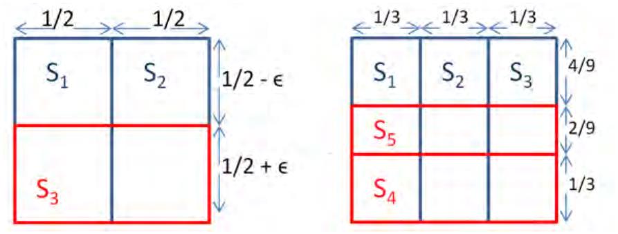

1
3
· 2 ·| |
U = U new elements. Thus we add a set S , disjoint from S , covering slightly
2| |
cover
5
4
3
9
2
more than a fraction of U. In the third iteration we allow the greedy algorithm to pick one
9
of S , S , S . The value of the greedy solution is ≈ |U|( + + ) = U . This is roughly
1
2
1 4
3 9
19| |
1
2
3
3
9
27
7
0% of |U|, so it is a worse example for the greedy algorithm than the first
Exercise Set #8 asks you to extend this family of bad examples to show that, for all k,
the greedy solution could be as small as
ꢀ
ꢁ
k
1
1
− 1 −
k
3
19
times the size of an optimal solution. (Note that with k = 2, 3 we get and .) This
1
4 27
63.2% in the limit (since 1
expression is decreasing with k, and approaches 1 −
≈
−
x
e
approaches e for x going to 0, recall Figure 5).4
−
x
1
0
5
y = e−
x
−
5
5
10
y = 1 − x
−
5
Figure 5: Graph showing 1 − x approaching e−x for small x.
These examples show that the following guarantee is remarkable.
Theorem 2.2 For every k ≥ 1, the greedy algorithm is a (1 − (1 − ) )-approximation
1
k
k
algorithm for set coverage instances with budget k.
Thus there are no worse examples for the greedy algorithm that the ones we identified
above. Here’s what’s even more amazing: under standard complexity assumptions, there is
no polynomial-time algorithm with a better approximation ratio!5 In this sense, the greedy
algorithm is an optimal approximation algorithm for the set coverage problem.
We now turn to the proof of Theorem 2.2. The following lemma proves a sense in which
the greedy algorithm makes healthy progress at every step. (This is the most common way
to analyze a greedy algorithm, whether for exact or approximate guarantees.)
4
5
There’s that strange number again!
As k grows large, that is. When k is a constant, the problem can be solved optimally in polynomial time
using brute-force search.
8


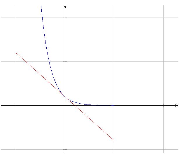

Lemma 2.3 Suppose that the first i − 1 sets A , . . . , A
computed by the greedy algorithm
1
cover ` elements. Then the next set A chosen be the algorithm covers at least
i−1
i
1
(OPT − `)
k
new elements, where OPT is the value of an optimal solution.
Proof: As a thought experiment, suppose that the greedy algorithm were allowed to pick k
new sets in this iteration. Certainly it could cover OPT − ` new elements — just pick all of
the k subsets in the optimal solution. One of these k sets must cover at least (OPT `)
−
1
k
new elements, and the set A chosen by the greedy algorithm is at least as good. ꢀ
i
Now we just need a little algebra to prove the approximation guarantee.
Proof of Theorem 2.2: Let g = | ∪i A | denote the number of elements covered by the
i
greedy solution after i iterations. Applying Lemma 2.3, we get
j=1
i
ꢀ
ꢁ
1
OPT
1
g = (g − gk−1) + gk−1 ≥ (OPT − gk−1) + gk−1
=
+ 1 −
gk−1
.
k
k
k
k
k
Applying it again we get
ꢀ
ꢁ ꢀ
ꢀ
ꢁ
ꢁ
ꢀ
ꢁ
ꢀ
ꢁ
2
OPT
k
1
OPT
k
1
OPT
k
1
OPT
k
1
gk ≥
+ 1 −
+ 1 −
gk−2
=
+ 1 −
+ 1 −
gk−3
.
k
k
k
k
Iterating, we wind up with
"
#
ꢀ
ꢁ
ꢀ
ꢁ
ꢀ
ꢁk−1
2
OPT
k
1
1
1
gk ≥
1 + 1 −
+ 1 −
+ · · · + 1 −
.
k
k
k
(There are k terms, one per iteration of the greedy algorithm.) Recalling from your discrete
math class the identity
1
− zk
− z
1
+ z + z2 + · · · + zk−1
=
1
for z ∈ (0, 1) — just multiply both sides by 1 − z to verify — we get
"
#
ꢀ
ꢁ
1
k
k
OPT 1 − (1 − )
1
gk ≥
·
k
= OPT 1
−
1
−
,
k
1 − (1 − 1 )
k
k
as desired. ꢀ
9


2
.5 Influence Maximization
Guarantees for the greedy algorithm for set coverage and various generalizations were already
known in the 1970s. But just over the last dozen years, these ideas have taken off in the
data mining and machine learning communities. We’ll just mention one representative and
influential (no pun intended) example, due to Kempe, Kleinberg, and Tardos in 2003.
Consider a “social network,” meaning a directed graph G = (V, E). For our purposes, we
interpret an edge (v, w) as “v influences w.” (For example, maybe w follows v on Twitter.)
We next posit a simple model of how an idea/news item/meme/etc. “goes viral,” called
a “cascade model.”6
•
•
Initially the vertices in some set S are “active,” all other vertices are “inactive.” Every
edge is initially “undetermined.”
While there is an active vertex v and an undetermined edge (v, w):
–
–
with probability p, edge (v, w) is marked “active,” otherwise it is marked “inac-
tive;”
if (v, w) is active and w is inactive, then mark w as active.
Thus whenever a vertex gets activated, it has the opportunity to active all of the vertices
that it influences (if they’re not already activated). Note that once a vertex is activated, it
is active forevermore. A vertex can get multiple chances to be activated, corresponding to
the number of its influencers who get activated. See Figure 6. In the example, note that a
vertex winds up getting activated if and only if there is a path of activated edges from v to
it.
a
c
b
d
Figure 6: Example cascade model. Initially, only a is activated. b (and similarly c) can get
activated by a with probability p. d has a chance to get activated by either a, b or c.
The influence maximization problem is, given a directed graph G = (V, E) and a budget k,
to compute the subset S ⊆ V of size k that maximizes the expected number of active vertices
at the conclusion of the cascade, given that the vertices of S are active at the beginning.
6
Such models were originally proposed in epidemiology, to understand the spread of diseases.
1
0
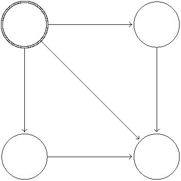

(The expectation is over the coin flips made for the edges.) Denote this expected value for
a set S by f(S).
There is a natural greedy algorithm for influence maximization, where at each iteration
we increase the function f as much as possible.
Greedy Algorithm for Influence Maximization
S = ∅
for i = 1, 2, . . . , k: do
add to S the vertex v maximizing f(S ∪ {v})
return S
The same analysis we used for set coverage can be used to prove that this greedy algorithm
1
is a (1 − (1 − ) )-approximation algorithm for influence maximization. The greedy algo-
k
k
rithm’s guarantee holds for every function f that is “monotone” and “submodular,” and the
function f above is one such example (it is basically a convex combination of set coverage
functions). See Problem Set #4 for details.
1
1


CS261: A Second Course in Algorithms
Lecture #16: The Traveling Salesman Problem∗
Tim Roughgarden†
February 25, 2016
1
The Traveling Salesman Problem (TSP)
In this lecture we study a famous computational problem, the Traveling Salesman Problem
(TSP). For roughly 70 years, the TSP has served as the best kind of challenge problem, mo-
tivating many different general approaches to coping with NP-hard optimization problems.
For example, George Dantzig (who you’ll recall from Lecture #10) spent a fair bit of his time
in the 1950s figuring out how to use linear programming as a subroutine to solve ever-bigger
instances of TSP. Well before the development of NP-completeness in 1971, experts were
well aware that the TSP is a “hard” problem in some sense of the word.
So what’s the problem? The input is a complete undirected graph G = (V, E), with a
nonnegative cost c ≥ 0 for each edge e ∈ E. By a TSP tour, we mean a simple cycle that
e
visits each vertex exactly once. (Not to be confused with an Euler tour, which uses each
edge exactly once.) The goal is to compute the TSP tour with the minimum total cost. For
example, in Figure 1, the optimal objective function value is 13.
The TSP gets its name from a silly story about a salesperson who has to make a number
of stops, and wants to visit them all in an optimal order. But the TSP definitely comes up in
real-world scenarios. For example, suppose a number of tasks need to get done, and between
two tasks there is a setup cost (from, say, setting up different equipment or locating different
workers). Choosing the order of operations so that the tasks get done as soon as possible is
exactly the TSP. Or think about a scenario where a disk has a number of outstanding read
requests; figuring out the optimal order in which to serve them again corresponds to TSP.
∗
†
ꢀc
2
Department of Computer Science, Stanford University, 474 Gates Building, 353 Serra Mall, Stanford,
016, Tim Roughgarden.
CA 94305. Email: tim@cs.stanford.edu.
1

c
3
5
1
4
2
6
a
b
d
Figure 1: Example TSP graph. Best TSP tour is a-c-b-d-a with cost 13.
The TSP is hard, even to approximate.
Theorem 1.1 If P = NP, then there is no α-approximation algorithm for the TSP (for
any α).
Recall that an α-approximation algorithm for a minimization problem runs in polynomial
time and always returns a feasible solution with cost at most α times the minimum possible.
Proof of Theorem 1.1: We prove the theorem using a reduction from the Hamiltonian cycle
problem. The Hamiltonian cycle problem is: given an undirected graph, does it contain a
simple cycle that visits every vertex exactly once? For example, the graph in Figure 2 does
not have a Hamiltonian cycle.1 This problem is NP-complete, and usually one proves it in
a course like CS154 (e.g., via a reduction from 3SAT).
a
c
f
i
b
e
d
g
h
Figure 2: Example graph without Hamiltonian cycle.
1
While it’s generally difficult to convince someone that a graph has no Hamiltonian cycle, in this case
there is a slick argument: color the four corners and the center vertex green, and the other four vertices
red. Then every closed walk alternates green and red vertices, so a Hamiltonian cycle would have the same
number of green and red vertices (impossible, since there are 9 vertices).
2
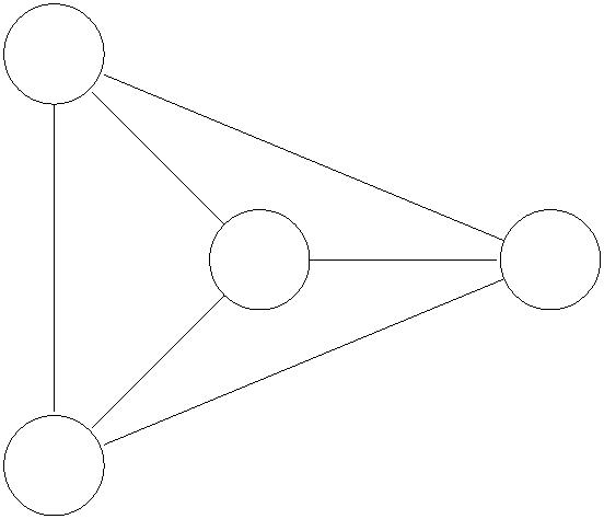
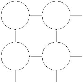
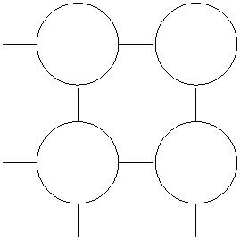
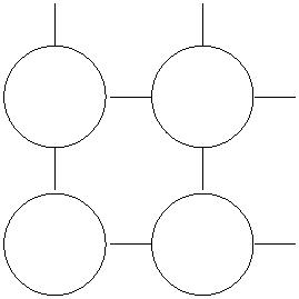

For the reduction, we need to show how to use a good TSP approximation algorithm to
solve the Hamiltonian cycle problem. Given an instance G = (V, E) of the latter problem,
0
we transform it into an instance G = (V , E , c) of TSP, where:
0
0
•
•
•
V 0 = V ;
E0 is all edges (so (V 0, E0) is the complete graph);
for each e ∈ E0, set
ꢀ
where n is the number of vertices and α is the approximation factor that we want to
rule out.
1
if e ∈ E
ce =
>
α · n if e ∈/ E,
For example, in Figure 2, all the edges of the grid get a cost of 1, and all the missing edges
get a cost greater than αn.
The key point is that there is a one-to-one correspondence between the Hamiltonian
cycles of G and the TSP tours of G0 that use only unit-cost edges. Thus:
(i) If G has a Hamiltonian cycle, then there is a TSP tour with total cost n.
(ii) If G has no Hamiltonian cycle, then every TSP tour has cost larger than αn.
Now suppose there were an α-approximation algorithm A for the TSP. We could use A to
solve the Hamiltonian cycle problem: given an instance G of the problem, run the reduction
above and then invoke A on the produced TSP instance. Since there is more than an α
factor gap between cases (i) and (ii) and A is an α-approximation algorithm, the output of
A indicates whether or not G is Hamiltonian. (If yes, then it must return a TSP tour with
cost at most αn; if no, then it can only return a TSP tour with cost bigger than αn.) ꢀ
2
Metric TSP
2
.1 Toward a Tractable Special Case
Theorem 1.1 indicates that, to prove anything interesting about approximation algorithms for
the TSP, we need to restrict to a special case of the problem. In the metric TSP, we assume
that the edge costs satisfy the triangle inequality (with cuw ≤ c + c for all u, v, w ∈ V ).
uv
vw
We previously saw the triangle inequality when studying the Steiner tree problem (Lectures
#
13 and #15). The big difference is that in the Steiner tree problem the metric assumption
is without loss of generality (see Exercise Set #7) while in the TSP it makes the problem
significantly easier.2
The metric TSP problem is still NP-hard, as shown by a variant of the proof of Theo-
rem 1.1. We can’t use the big edge costs αn because this would violate the triangle inequality.
2
This is of course what we’re hoping for, because the general case is impossible to approximate.
3

But if we use edge costs of 2 for edges not in the given Hamiltonian cycle instance G, then
the triangle inequality holds trivially (why?). The optimal TSP tour still has value at most
n when G has a Hamiltonian cycle, and value at least n + 1 when it does not. This shows
that there is no exact polynomial-time algorithm for metric TSP (assuming P = NP). It
does not rule out good approximation algorithms, however. And we’ll see next that there
are pretty good approximation algorithms for metric TSP.
2
.2 The MST Heuristic
Recall that in approximation algorithm design and analysis, the challenge is to relate the
solution output by an algorithm to the optimal solution. The optimal solution itself is often
hard to get a handle on (its NP-hard to compute, after all), so one usually resorts to bounds
on the optimal objective function value — quantities that are “only better than optimal.”
Here’s a simple lower bound for the TSP, with or without the triangle inequality.
Lemma 2.1 For every instance G = (V, E, c), the minimum-possible cost of a TSP tour is
at least the cost of a minimum spanning tree (MST).
Proof: Removing an edge from the minimum-cost TSP tour yields a spanning tree with only
less cost. The minimum spanning tree can only have smaller cost. ꢀ
Lemma 2.1 motivates using the MST as a starting point for building a TSP tour — if
we can turn the MST into a tour without suffering too much extra cost, then the tour will
be near-optimal. The idea of transforming a tree into a tour should ring some bells — recall
our online (Lecture #13) and offline (Lecture #15) algorithms for the Steiner tree problem.
We’ll reuse the ideas developed for Steiner tree, like doubling and shortcutting, here for the
TSP. The main difference is that while these ideas were used only in the analysis of our
Steiner tree algorithms, to relate the cost of our algorithm’s tree to the minimum-possible
cost, here we’ll use these ideas in the algorithm itself. This is because, in TSP, we have to
output a tour rather than a tree.
MST Heuristic for Metric TSP
compute the MST T of the input G
construct the graph H by doubling every edge of T
compute an Euler tour C of H
// every v ∈ V is visited at least once in C
shortcut repeated occurrences of vertices in C to obtain a TSP tour
When we studied the Steiner tree problem, steps 2–4 were used only in the analysis. But
all of these steps, and hence the entire algorithm, are easy to implement in polynomial (even
near-linear) time.3
3
Recall from CS161 that there are many fast algorithms for computing a MST, including Kruskal’s and
Prim’s algorithms.
4


Theorem 2.2 The MST heuristic is a 2-approximation algorithm for the metric TSP.
Proof: We have
cost of our TSP tour ≤ cost of C
X
=
c
e
e∈H
2
X
=
ce
e∈T
≤
2 · cost of optimal TSP tour,
where the first inequality holds because the edge costs obey the triangle inequality, the
second equation holds because the Euler tour C uses every edge of H exactly once, the third
equation follows from the definition of H, and the final inequality follows from Lemma 2.1.
ꢀ
The analysis of the MST heuristic in Theorem 2.2 is tight — for every constant c < 2,
there is a metric TSP instance such that the MST heuristic outputs a tour with cost more
than c times that of an optimal tour (Exercise Set #8).
Can we do better with a different algorithm? This is the subject of the next section.
2
.3 Christofides’s Algorithm
Why were we off by a factor of 2 in the MST heuristic? Because we doubled every edge of
the MST T. Why did we double every edge? Because we need an Eulerian graph, to get
an Euler tour that we can shortcut down to a TSP tour. But perhaps it’s overkill to double
every edge of the MST. Can we augment the MST T to get an Eulerian graph without paying
the full cost of an optimal solution?
The answer is yes, and the key is the following slick lemma. It gives a second lower bound
on the cost of an optimal TSP tour, complementing Lemma 2.1.
Lemma 2.3 Let G = (V, E) be a metric TSP instance. Let S ⊆ V be an even subset of
vertices and M a minimum-cost perfect matching of the (complete) graph induced by S. Then
X
1
ce ≤ · OP T,
2
e∈M
where OPT denotes the cost of an optimal TSP tour.
Proof: Fix S. Let C∗ denote an optimal TSP tour. Since the edges obey the triangle
inequality, we can shortcut C to get a tour C of S that has cost at most OPT. Since |S| is
∗
S
even, C is a (simple) cycle of even length (Figure 3). C is the union of two disjoint perfect
S
S
matchings (alternate coloring the edges of CS red and green). Since the sum of the costs of
these matchings is that of C (which is at most OPT), the cheaper of these two matchings
S
has cost at most OP T/2. The minimum-cost perfect matching of S can only be cheaper. ꢀ
5

a
e
b
f
c
d
Figure 3: CS is a simple cycle of even length representing union of two disjoint perfect
matchings (red and green).
Lemma 2.3 brings us to Christofides’s algorithm, which differs from the MST heuristic
only in substituting a perfect matching computation in place of the doubling step.
Christofides’s Algorithm
compute the MST T of the input G
compute the set W of vertices with odd degree in T
compute a minimum-cost perfect matching M of W
construct the graph H by adding M to T
compute an Euler tour C of H
// every v ∈ V is visited at least once in C
shortcut repeated occurrences of vertices in C to obtain a TSP tour
In the second step, the set W always has even size. (The sum of the vertex degrees of a graph
is double the number of edges, so there cannot be an odd number of odd-degree vertices.) In
the third step, note that the relevant matching instance is the graph induced by W, which
is the complete graph on W. Since this is not a bipartite graph (at least if |W| ≥ 4), this is
an instance of nonbipartite matching. We haven’t covered any algorithms for this problem,
but we mentioned in Lecture #6 that the ideas behind the Hungarian algorithm (Lecture
#
5) can, with additional ideas, be extended to also solve the nonbipartite case in polynomial
time. In the fourth step, there may be edges that appear in both T and M. The graph H
contains two copies of such edges, which is not a problem for us. The last two steps are
the same as in the MST heuristic. Note that the graph H is indeed Eulerian — adding the
matching M to T increases the degree of each vertex v ∈ W by exactly one (and leaves other
degrees unaffected), so T + M has all even degrees.4 This algorithm can be implemented in
polynomial time — the overall running time is dominated by the matching computation in
the third step.
3
Theorem 2.4 Christofides’s algorithm is a -approximation algorithm for the metric TSP.
2
4
And as usual, H is connected because T is connected.
6


Proof: We have
cost of our TSP tour ≤ cost of C
X
=
c
e
e∈H
X
X
=
ce
+
ce
e∈T
e∈M
|
{z }
| {z }
≤
OPT (Lem 2.1)
≤OPT/2 (Lem 2.3)
3
≤
· cost of optimal TSP tour,
2
where the first inequality holds because the edge costs obey the triangle inequality, the
second equation holds because the Euler tour C uses every edge of H exactly once, the third
equation follows from the definition of H, and the final inequality follows from Lemmas 2.1
and 2.3. ꢀ
The analysis of Christofides’s algorithm in Theorem 2.4 is tight — for every constant
3
c < , there is a metric TSP instance such that the algorithm outputs a tour with cost more
than c times that of an optimal tour (Exercise Set #8).
2
Christofides’s algorithm is from 1976. Amazingly, to this day we still don’t know whether
or not there is an approximation algorithm for metric TSP better than Christofides’s algo-
rithm. It’s possible that no such algorithm exists (assuming P = NP, since if P = NP the
4
problem can be solved optimally in polynomial time), but it is widely conjecture that (if
not better) is possible. This is one of the biggest open questions in the field of approximation
algorithms.
3
3
Asymmetric TSP
a
d
b
c
Figure 4: Example ATSP graph. Note that edges going in opposite directions need not have
the same cost.
We conclude with an approximation algorithm for the asymmetric TSP (ATSP) problem,
the directed version of TSP. That is, the input is a complete directed graph, with an edge
7


in each direction between each pair of vertices, and a nonnegative cost c ≥ 0 for each edge
e
(Figure 4). The edges going in opposite directions between a pair of vertices need not have
the same cost.5 The “normal” TSP is equivalent to the special case in which opposite edges
(between the same pair of vertices) have the same cost. The goal is to compute the directed
TSP tour — a simple directed cycle, visiting each vertex exactly once — with minimum-
possible cost. Since the ATSP includes the TSP as a special case, it can only harder (and
appears to be strictly harder). Thus we’ll continue to assume that the edge costs obey the
triangle inequality (cuw ≤ c +c for every u, v, w ∈ V ) — note that this assumption makes
uv
vw
perfect sense in directed graphs as well as undirected graphs.
Our high-level strategy mirrors that in our metric TSP approximation algorithms.
1
2
. Construct a not-too-expensive Eulerian directed graph H.
. Shortcut H to get a directed TSP tour; by the triangle inequality, the cost of this tour
is at most
P
c .
e
e∈H
Recall that a directed graph H is Eulerian if (i) it is strongly connected (i.e., for every v, w
there is a directed path from v to w and also a directed path from w to v); and (ii) for
every vertex v, the in-degree of v in H equals its out-degree in H. Every directed Eulerian
graph admits a directed Euler tour — a directed closed walk that uses every (directed) edge
exactly once. Assumptions (i) and (ii) are clearly necessary for a graph to have a directed
Euler tour (since one enters and exists a vertex the same number of times). The proof of
sufficiency is basically the same as in the undirected case (cf., Exercise Set #7).
The big question is how to implement the first step of constructing a low-cost Eulerian
graph. In the metric case, we used the minimum spanning tree as a starting point. In the
directed case, we’ll use a different subroutine, for computing a minimum-cost cycle cover.
a
d
e
f
g
b
c
i
h
Figure 5: Example cycle cover of vertices.
A cycle cover of a directed graph is a collection of C , . . . , C of directed cycles, each
1
k
with at least two vertices, such that each vertex v ∈ V appears in exactly one of the cycles.
(This is, the cycles partition the vertex set.) See Figure 5. Note that directed TSP tours
5
Recalling the motivating scenario of scheduling the order of operations to minimize the overall setup
time, it’s easy to think of cases where the setup time between task i and task j is not the same as if the
order of i and j are reversed.
8
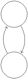
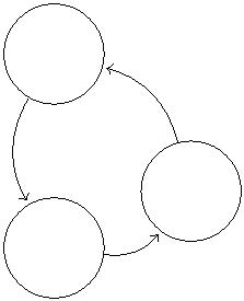

are exactly the cycle covers with k = 1. Thus, the minimum-cost cycle cover can only be
cheaper than the minimum-cost TSP tour.
Lemma 3.1 For every instance G = (V, E, c) of ATSP, the minimum-possible cost of a
directed TSP tour is at least that of a minimum-cost cycle cover.
The minimum-cost cycle cover of a directed graph can be computed in polynomial time. This
is not obvious, but as a student in CS261 you’re well-equipped to prove it (via a reduction
to minimum-cost bipartite perfect matching, see Problem Set #4).
Approximation Algorithm for ATSP
initialize F = ∅
initialize G to the input graph
while G has at least 2 vertices do
compute a minimum-cost cycle cover C , . . . , C of the current G
1
k
add to F the edges in C1, . . . , Ck
for i = 1, 2, . . . , k do
delete from G all but one vertex from Ci
compute a directed Euler tour C of H = (V, F)
// H is Eulerian, see discussion below
shortcut repeated occurrences of vertices on C to obtain a TSP tour
For the last two steps of the algorithm to make sense, we need the following claim.
Claim: The graph H = (V, F) constructed by the algorithm is Eulerian.
Proof: Note that H = (V, F) is the union of all the cycle covers computed over all iterations
of the while loop. We prove two invariants of (V, F) over these iterations.
First, the in-degree and out-degree of a vertex are always the same in (V, F). This is
trivial at the beginning, when F = ∅. When we add in the first cycle cover to F, every vertex
then has in-degree and out-degree equal to 1. The vertices that get deleted never receive
any more incoming or outgoing edges, so they have the same in-degree and out-degree at the
conclusion of the while loop. The undeleted vertices participate in the cycle cover computed
in the second iteration; when this cycle cover is added to H, the in-degree and out-degree
of each vertex in (V, F) increases by 1 (from 1 to 2). And so on. At the end, the in- and
out-degree of a vertex v is exactly the number of while loop iterations in which it participated
(before getting deleted).
Second, at all times, for all vertices v that have been deleted so far, there is a vertex w
that has not yet been deleted such that (V, F) contains both a directed path from v to w
and from w to v. That is, in (V, F), every deleted vertex can reach and be reached by some
undeleted vertex.
To see why this second invariant holds, consider the first iteration. Every deleted vertex
v belongs to some cycle C of the cycle cover, and some vertex w on C was left undeleted. C
i
i
i
9

contains a directed path from v to w and vice versa, and F contains all of Ci. By the same
reasoning, every vertex v that was deleted in the second iteration has a path in (V, F) to and
from some vertex w that was not deleted. A vertex u that was deleted in the first iteration
has, at worst, paths in (V, F) to and from a vertex v deleted in the second iteration; stitching
these paths together with the paths from v to an undeleted vertex w, we see that (V, F)
contains a path from u to this undeleted vertex w, and vice versa. In the final iteration of
the while loop, the cycle cover contains only one cycle C. (Otherwise, at least 2 vertices
would not be deleted and the while loop would continue.) The edges of C allow every vertex
remaining in the final iteration to reach every other such vertex. Since every deleted vertex
can reach and be reached by the vertices remaining in the final iteration, the while loops
concludes with a graph (V, F) where everybody can reach everybody (i.e., which is strongly
connected). ꢀ
The claim implies that our ATSP algorithm is well defined. We now give the easy
argument bounding the cost of the tour it produces.
Lemma 3.2 In every iteration of the algorithm’s main while loop, there exists a directed
TSP tour of the current graph G with cost at most OPT, the minimum cost of a TSP tour
in the original input graph.
Proof: Shortcutting the optimal TSP tour for the original graph down to one on the current
graph G yields a TSP tour with cost at most OPT (using the triangle inequality). ꢀ
By Lemmas 3.1 and 3.2:
Corollary 3.3 In every iteration of the algorithm’s main while loop, the cost of the edges
added to F is at most OPT.
Lemma 3.4 There are at most log2 n iterations of the algorithm’s main while loop.
Proof: Recall that every cycle in a cycle cover has, by definition, at least two vertices. The
algorithm deletes all but one vertex from each cycle in each iteration, so it deletes at least
one vertex for each vertex that remains. Since the number of remaining vertices drops by a
factor of at least 2 in each iteration, there can only be log2 n iterations. ꢀ
Corollary 3.3 and Lemma 3.4 immediately give the following.
Theorem 3.5 The ATSP algorithm above is a log2 n-approximation algorithm.
This algorithm is from the early 1980s, and progress since then has been modest. The
best-known approximation algorithm for ATSP has an approximation ratio of O(log n/ log log n),
and even this improvement is only from 2010! Another of the biggest open questions in all of
approximation algorithms is: is there a constant-factor approximation algorithm for ATSP?
1
0
CS261: A Second Course in Algorithms
Lecture #17: Linear Programming and Approximation
Algorithms∗
Tim Roughgarden†
March 1, 2016
1
Preamble
Recall that a key ingredient in the design and analysis of approximation algorithms is getting
a handle on the optimal solution, to compare it to the solution return by an algorithm. Since
the optimal solution itself is often hard to understand (it’s NP-hard to compute, after all),
this generally entails bounds on the optimal objective function value — quantities that are
“only better than optimal.” If the output of an algorithm is within an α factor of this bound,
then it is also within an α factor of optimal.
So where do such bounds on the optimal objective function value come from? Last
week, we saw a bunch of ad hoc examples, including the maximum job size and the average
load in the makespan-minimization problem, and the minimum spanning tree for the metric
TSP. Today we’ll see how to use linear programs and their duals to generate systematically
such bounds. Linear programming and approximation algorithms are a natural marriage
—
for example, recall that dual feasible solutions are by definition bounds on the best-
possible (primal) objective function value. We’ll see that some approximation algorithms
explicitly solve a linear program; some use linear programming to guide the design of an
algorithm without ever actually solving a linear program to optimality; and some use linear
programming duality to analyze the performance of a natural (non-LP-based) algorithm.
2
A Greedy Algorithm for Set Cover (Without Costs)
We warm up with a solution that builds on our set coverage greedy algorithm (Lecture #15)
and doesn’t require linear programming at all. In the set cover problem, the input is a list
∗
†
ꢀc
2
Department of Computer Science, Stanford University, 474 Gates Building, 353 Serra Mall, Stanford,
016, Tim Roughgarden.
CA 94305. Email: tim@cs.stanford.edu.
1

S , . . . , S ⊆ U of sets, each specified as a list of elements from a ground set U. The goal
1
m
is to pick as few sets as possible, subject to the constraint their union is all of U (i.e., that
they form a set cover). For example, in Figure 1, the optimal solution comprises of picking
the blue sets.
Figure 1: Example set coverage problem. The optimal solution comprises of picking the blue
sets.
In the set coverage problem (Lecture #15), the input included a parameter k. The
hard constraint was to pick at most k sets, and subject to this the goal was to cover as
many elements as possible. Here, the constraint and the objective are reversed: the hard
constraint is to cover all elements and, subject to this, to use as few sets as possible. Potential
applications of the set cover problem are the same as for set coverage, and which problem
is a better fit for reality depends on the context. For example, if you are choosing where to
build fire stations, you can imagine that it’s a hard constraint to have reasonable coverage
of all of the neighborhoods of a city.
The set cover problem is NP-hard, for essentially the same reasons as the set coverage
problem. There is again a tension between the size of a set and how “redundant” it is with
other sets that might get chosen anyway.
Turning to approximation algorithms we note that the greedy algorithm for set coverage
makes perfect sense for set cover. The only difference is in the stopping condition — rather
than stopping after k iterations, the algorithm stops when it has found a set cover.
Greedy Algorithm for Set Cover (No Costs)
C = ∅
while C not a set cover do
add to C the set S which covers the largest number of new elements
i
/ elements covered by previously chosen sets don’t count
/
return C
The same bad examples from Lecture #15 show that the greedy algorithm is not in
general optimal. In the first example of that lecture, the greedy algorithm uses 3 sets even
2
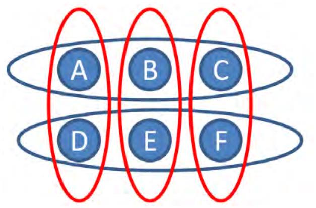

though 2 are enough; in the second lecture, it uses 5 sets even though 3 are enough. (And
there are worse examples than these.) We next prove an approximation guarantee for the
algorithm.
Theorem 2.1 The greedy algorithm is a ln n-approximation algorithm for the set cover prob-
lem, where n = |U| is the size of the ground set.
Proof: We can usefully piggyback on our analysis of the greedy algorithm for the set coverage
problem (Lecture #15). Consider a set cover instance, and let OPT denote the size of the
smallest set cover. The key observation is: the current solution after OPT iterations of the
set cover greedy algorithm is the same as the output of the set coverage greedy algorithm
with a budget of k = OPT. (In both cases, in every iteration, the algorithm picks the set
that covers the maximum number of new elements.) Recall from Lecture #15 that the greedy
algorithm is a (1 − )-approximation algorithm for set coverage. Since there is a collection
1
e
of OPT sets covering all |U| elements, the greedy algorithm, after OPT iterations, will have
covered at least (1 − ) U elements, leaving at most U /e elements uncovered. Iterating,
1
e
| |
| |
every OPT iterations of the greedy algorithm will reduce the number of uncovered elements
by a factor of e. Thus all elements are covered within OPT loge n = OPT ln n iterations.
Thus the number of sets chosen by the greedy algorithm is at most ln n times the size of an
optimal set cover, as desired. ꢀ
3
A Greedy Algorithm for Set Cover (with Costs)
It’s easy to imagine scenarios where the different sets of a set cover instance have different
costs. (E.g., if sets model the skills of potential hires, different positions/seniority may
command different salaries.) In the general version of the set cover problem, each set Si also
has a nonnegative cost c ≥ 0. Since there were no costs in the set coverage problem, we can
i
no longer piggyback on our analysis there — we’ll need a new idea.
The greedy algorithm is easy to extend to the general case. If one set costs twice as much
as another, then to be competitive, it should cover at least twice as many elements. This
idea translates to the following algorithm.
Greedy Algorithm for Set Cover (With Costs)
C = ∅
while C not a set cover do
add to C the set S with the minimum ratio
i
ci
newly covered elements
ri =
(1)
#
return C
3


Note that if all of the ci’s are identical, then we recover the previous greedy algorithm —
in this case, minimizing the ratio is equivalent to maximizing the number of newly covered
elements. In general, the ratio is the “average cost per-newly covered element,” and it makes
sense to greedily minimize this.
The best-case scenario is that the approximation guarantee for the greedy algorithm does
not degrade when we allow arbitrary set costs. This is indeed the case.
Theorem 3.1 The greedy algorithm is a ≈ ln n-approximation algorithm for the general set
cover problem (with costs), where n = |U| is the size of the ground set.1
To prove Theorem 3.1, the first order of business is to understand how to make use of
the greedy nature of the algorithm. The following simple lemma, reminiscent of a lemma in
Lecture #15 for set coverage, addresses this point.
Lemma 3.2 Suppose that the current greedy solution covers ` elements of the set Si. Then
the next set chosen by the algorithm has ratio at most
ci
.
(2)
|
Si| − `
Indeed, choosing the set Si would attain the ratio in (2); the ratio of the set chosen by the
greedy algorithm can only be smaller.
For every element e ∈ U, define
qe = ratio of the first set chosen by the greedy algorithm that covers e.
Since the greedy algorithm terminates with a set cover, every element has a well-defined
q-value.2 See Figure 2 for a concrete example.
Figure 2: Example set with q-value of the elements.
1
Inspection of the proof shows that the approximation ratio is ≈ ln s, where s = max |S | is the maximum
i
i
size of an input set.
2
The notation is meant to invoke the q-values in our online bipartite matching analysis (Lecture #13);
as we’ll see, something similar is going on here.
4

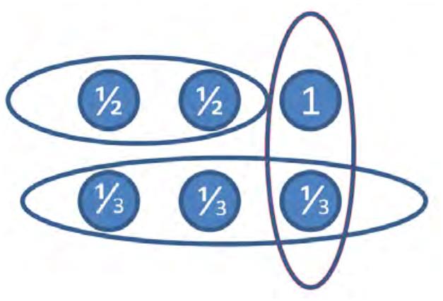

Corollary 3.3 For every set S , the jth element e of S to be covered by the greedy algorithm
i
i
satisfies
ci
Si| − (j − 1)
qe ≤
.
(3)
|
Corollary 3.3 follows immediately from Lemma 3.2 in the case where the elements of Si are
covered one-by-one (with j − 1 playing the role of `, for each j). In general, several elements
of S might be covered at once. (E.g., the greedy algorithm might actually pick S .) But
i
i
in this case the corollary is only “more true” — if j is covered as part of a batch, then
the number of uncovered elements in S before the current selection was j − 1 or less. For
i
example, in Figure 2, Corollary 3.3 only asserts that the q-values of the largest set are at
1
1
2
1
most , , and 1, when in fact all are only . Similarly, for the last set chosen, Corollary 3.3
1
3
3
only guarantees that the q-values are at most and 1, while in fact they are and 1.
1
2
We can translate Corollary 3.3 into a bound on the sum of the q-values of the elements
3
of a set Si:
X
ci
ci
ci ci
qe ≤
+
+ · · · +
+
|
Si| |Si| − 1
2
1
e∈S
i
≈
≤
c ln |S |
(4)
(5)
i
i
c ln n,
i
where n = |U| is the ground set size.3
We also have
X
qe = cost of the greedy set cover.
(6)
e∈U
This identity holds inductively at all times. (If e has not been covered yet, then we define
q = 0.) Initially, both sides are 0. When a new set S is chosen by the greedy algorithm,
e
i
the right-hand side goes up by ci. The left-hand side also increases, because all of the newly
covered elements receive a q-value (equal to the ratio of the set Si), and this increase is
r · (# of newly covered elements) = c .
i
i
(Recall the definition (1) of the ratio.)
Proof of Theorem 3.1: Let {S , . . . , S denote the sets of an optimal set cover, and OPT
∗
∗}
1
k
P|
S |
3
Our estimate
i
1
≈ ln |S | in (4), which follows by approximating the sum by an integral, is actually
j=1 j
off by an additive constant less that 1 (known as “Euler’s constant”). We ignore this additive constant for
i
simplicity.
5


its cost. We have
X
cost of the greedy set cover =
qe
e∈U
Xk X
≤
qe
i=1 e∈S∗
i
Xk
≤
ci ln n
i=1
=
OPT · ln n,
∗
∗
k
where the first equation is (6), the first inequality follows because S , . . . , S form a set cover
1
(each e ∈ U is counted at least once), and the second inequality from (5). This completes
the proof. ꢀ
Our analysis of the greedy algorithm is tight. To see this, let U = {1, 2, . . . , n}, S = U
0
with c = 1 + ꢀ for small ꢀ, and S = {i} with cost c = for i = 1, 2, . . . , n. The optimal
1
i
0
i
i
solution (S ) has cost 1 + ꢀ. The greedy algorithm chooses S , Sn−1, . . . , S1 (why?), for a
0
total cost of
P
n
n
1
≈ ln n.
i=1 i
More generally, the approximation factor of ≈ ln n cannot be beaten by any polynomial-
time algorithm, no matter how clever (under standard complexity assumptions). In this
sense, the greedy algorithm is optimal for the set cover problem.
4
Interpretation via Linear Programming Duality
Our proof of Theorem 3.1 is reasonably natural — using the greedy nature of the algorithm
to prove the easy Lemma 3.2 and then compiling the resulting upper bounds via (5) and (6)
— but it still seems a bit mysterious in hindsight. How would one come up with this type
of argument for some other problem?
We next re-interpret the proof of Theorem 3.1 through the lens of linear programming
duality. With this interpretation, the proof becomes much more systematic. Indeed, it
follows exactly the same template that we already used in Lecture #13 to analyze the
WaterLevel algorithm for online bipartite matching.
To talk about a dual, we need a primal. So consider the following linear program (P):
Xm
min
cixi
i=1
subject to
X
xi ≥ 1
xi ≥ 0
for all e ∈ U
for all Si.
i : e∈S
i
6

The intended semantics is for x to be 1 if the set S is chosen in the set cover, and 0
i
i
otherwise.4 In particular, every set cover corresponds to a 0-1 solution to (P) with the same
objective function value, and conversely. For this reason, we call (P) a linear programming
relaxation of the set cover problem — it includes all of the feasible solutions to the set cover
instance (with the same cost), in additional to other (fractional) feasible solutions. Because
the LP relaxation minimizes over a superset of the feasible set covers, its optimal objective
function value (“fractional OPT”) can only be smaller than that of a minimum-cost set cover
(“OPT”):
fractional OPT ≤ OP T.
We’ve seen a couple of examples of LP relaxations that are guaranteed to have optimal
-1 solutions — for the minimum s-t cut problem (Lecture #8) and for bipartite matching
0
(Lecture #9). Here, because the set cover problem is NP-hard and the linear programming
relaxation can be solved in polynomial time, we don’t expect the optimal LP solution to
always be integral. (Whenever we get lucky and the optimal LP solution is integral, it’s
handing us the optimal set cover on a silver platter.) It’s useful to see a concrete example of
this. In Figure 3, the ground set has 3 elements and the sets are the subsets with cardinality 2.
All costs are 1. The minimum cost of a set cover is clearly 2 (no set covers everything). But
1
setting xi = for every set yields a feasible fractional solution with the strictly smaller
2
objective function value of .
3
2
Figure 3: Example where all sets have cost 1. Optimal set cover is clearly 2, but there exists
3
2
1
2
a feasible fraction with value by setting all x = .
i
Deriving the dual (D) of (P) is straightforward, using the standard recipe (Lecture #8):
X
max
pe
e∈U
4
If you’re tempted to also include the constraints x ≤ 1 for every S , note that these will hold anyways
i
i
at an optimal solution.
7


subject to
X
pe ≤ ci
pe ≥ 0
for every set Si
for every e ∈ U.
e∈S
i
Lemma 4.1 If {pe}e∈E is a feasible solution to (D), then
X
pe ≤ fractional OPT ≤ OP T.
e∈U
The first inequality follows from weak duality — for a minimization problem, every feasible
dual solution gives (by construction) a lower bound on the optimal primal objective function
value — and second inequality follows because (P) is a LP relaxation of the set cover problem.
Recall the derivation from Section 3 that, for every set Si,
X
q ≤ c ln n;
e
i
e∈S
i
see (5). Looking at the constraints in the dual (D), the purpose of this derivation is now
transparent:
q
ln n
Lemma 4.2 The vector p :=
is feasible for the dual (D).
P
As such, the dual objective function value
cost of a set cover (Lemma 4.1).5 Using the identity (6) from Section 3, we get
pe provides a lower bound on the minimum
e∈U
X
cost of the greedy set cover = ln n ·
pe ≤ ln n · OP T.
e∈U
So, while one certainly doesn’t need to know linear programming to come up with the
greedy set cover algorithm, or even to analyze it, linear programming duality renders the
analysis transparent and reproducible for other problems. We next examine a couple of
algorithms whose design is explicitly guided by linear programming.
5
A Linear Programming Rounding Algorithm for Ver-
tex Cover
Recall from Problem Set #2 the vertex cover problem: the input is an undirected graph
G = (V, E) with a nonnegative cost c for each vertex v ∈ V , and the goal is to compute
v
a minimum-cost subset S ⊆ V that contains at least one endpoint of every edge. On
5
This is entirely analogous to what happened in Lecture #13, for maximum bipartite matching: we
defined a vector q with sum equal to the size of the computed matching, and we scaled up q to get a feasible
dual solution and hence an upper bound on the maximum-possible size of a matching.
8


Problem Set #2 you saw that, in bipartite graphs, this problem reduces to a max-flow/min-
cut computation. In general graphs, the problem is NP-hard.
The vertex cover problem can be regarded as a special case of the set cover problem. The
elements needing to be covered are the edges. There is one set per vertex v, consisting of the
edges incident to v (with cost cv). Thus, we’re hoping for an approximation guarantee better
than what we’ve already obtained for the general set cover problem. The first question to
ask is: does the greedy algorithm already have a better approximation ratio when we restrict
attention to the special case of vertex cover instances? The answer is no (Exercise Set #9),
so to do better we’ll need a different algorithm.
This section analyzes an algorithm that explicitly solves a linear programming relax-
ation of the vertex cover problem (as opposed to using it only for the analysis). The LP
relaxation (P) is the same one as in Section 4, specialized to the vertex cover problem:
X
min
cvxv
v∈V
subject to
x + x ≥ 1
for all e = (v, w) ∈ E
for all v ∈ V .
v
w
x ≥ 0
v
There is a one-to-one and cost-preserving correspondence between 0-1 feasible solutions to
this linear program and vertex covers. ( We won’t care about the dual of this LP relaxation
until the next section.)
Again, because the vertex cover problem is NP-hard, we don’t expect the LP relaxation
to always solve to integers. We can reinterpret the example from Section 4 (Figure 3) as a
vertex cover instance — the graph G is a triangle (all unit vertex costs), the smallest vertex
1
cover has size 2, but setting xv = for all three vertices yields a feasible fractional solution
2
3
2
with objective function value .
LP Rounding Algorithm for Vertex Cover
compute an optimal solution x∗ to the LP relaxation (P)
return S = {v ∈ V : xv
∗
≥ 12}
The first step of our new approximation algorithm computes an optimal (fractional)
solution to the LP relaxation (P). The second step transforms this fractional feasible solution
into an integral feasible solution (i.e., a vertex cover). In general, such a procedure is
called a rounding algorithm. The goal is to round to an integral solution without affecting
the objective function value too much.6 The simplest approach to LP rounding, and a
6
This is analogous to our metric TSP algorithms, where we started with an infeasible solution that was
only better than optimal (the MST) and then transformed it into a feasible solution (i.e., a TSP tour) with
suffering too much extra cost.
9


common heuristic in practice, is to round fractional values to the nearest integer (subject
to feasibility). The vertex cover problem is a happy case where this heuristic gives a good
worst-case approximation guarantee.
Lemma 5.1 The LP rounding algorithm above outputs a feasible vertex cover S.
∗
∗
∗ ≥
1 for every (v, w) E. Hence, for
∈
Proof: Since the solution x is feasible for (P), x + x
1
v
w
every (v, w) ∈ E, at least one of x , x is at least . Hence at least one endpoint of every
∗
∗
v
w
2
edge is included in the final output S. ꢀ
The approximation guarantee follows from the fact that the algorithm pays at most twice
what the optimal LP solution x∗ pays.
Theorem 5.2 The LP rounding algorithm above is a 2-approximation algorithm.
Proof: We have
X
X
∗
v
cv
≤
c (2x )
v
v∈S
v∈V
|
{z }
cost of alg’s soln
=
2 · fractional OPT
2 · OP T,
≤
where the first inequality holds because v ∈ S only if xv 2, the equation holds because x∗ is
an optimal solution to (P), and the second inequality follows because (P) is a LP relaxation
of the vertex cover problem. ꢀ
∗
≥ 1
6
A Primal-Dual Algorithm for Vertex Cover
Can we do better than Theorem 5.2? In terms of worst-case approximation ratio, the answer
seems to be no.7 But we can still ask if we can improve the running time. For example,
can we get a 2-approximation algorithm without explicitly solving the linear programming
relaxation? (E.g., for set cover, we used linear programs only in the analysis, not in the
algorithm itself.)
Our plan is to use the LP relaxation (P) and its dual (below) to guide the decisions made
by our algorithm, without ever solving either linear program explicitly (or exactly). The
dual linear program (D) is again just a specialization of that for the set cover problem:
X
max
pe
e∈E
7
Assuming the “Unique Games Conjecture,” a significant strengthening of the P = NP conjecture, there
is no (2 − ꢀ)-approximation algorithm for vertex cover, for any constant ꢀ > 0.
1
0


subject to
X
pe ≤ cv
pe ≥ 0
for every v ∈ V
for every e ∈ E.
e∈δ(v)
We consider the following algorithm, which maintains a dual feasible solution and itera-
tively works toward a vertex cover.
Primal-Dual Algorithm for Vertex Cover
initialize p = 0 for every edge e ∈ E
e
initialize S = ∅
while S is not a vertex cover do
pick an edge e = (v, w) with v, w ∈/ S
increase p until the dual constraint corresponding to v or w goes
e
tight
add the vertex corresponding to the tight dual constraint to S
In the while loop, such an edge (v, w) ∈ E must exist (otherwise S would be a vertex
cover). By a dual constraint “going tight,” we mean that it holds with equality. It is easy to
implement this algorithm, using a single pass over the edges, in linear time. This algorithm
is very natural when you’re staring at the primal-dual pair of linear programs. Without
knowing these linear programs, it’s not clear how one would come up with it.
For the analysis, we note three invariants of the algorithm.
(P1) p is feasible for (D). This is clearly true at the beginning when p = 0 for every e ∈ E
e
(vertex costs are nonnegative), and the algorithm (by definition) never violates a dual
constraint in subsequent iterations.
P
(P2) If v ∈ S, then
p = c . This is obviously true initially, and we only add a vertex
e∈δ(v)
e
to S when this condition holds for it.
v
(P3) If p > 0 for e = (v, w) ∈ E, then |S ∩ {v, w}| ≤ 2. This is trivially true (whether or
e
not p > 0).
e
Furthermore, by the stopping condition, at termination we have:
(P4) S is a vertex cover.
That is, the algorithm maintains dual feasibility and works toward primal feasibility. The
second and third invariants should be interpreted as an approximate version of the comple-
mentary slackness conditions.8 The second invariant is exactly the first set of complemen-
8
Recall the complementary slackness conditions from Lecture #9: (i) whenever a primal variable is
nonzero, the corresponding dual constraint is tight; (ii) whenever a dual variable is nonzero, the corresponding
primal constraint is tight. Recall that the complementary slackness conditions are precisely the conditions
under which the derivation of weak duality holds with equality. Recall that a primal-dual pair of feasible
solutions are both optimal if and only if the complementary slackness conditions hold.
1
1


tary slackness conditions — it says that a primal variable is positive (i.e., v ∈ S) only if
the corresponding dual constraint is tight. The second set of exact complementary slackness
conditions would assert that whenever p > 0 for e = (v, w) ∈ E, the corresponding primal
e
constraint is tight (i.e., exactly one of v, w is in S). These conditions will not in general hold
for the algorithm above (if they did, then the algorithm would always solve the problem ex-
actly). They do hold approximately, in the sense that tightness is violated only by a factor
of 2. This is exactly where the approximation factor of the algorithm comes from.
Since the algorithm maintains dual feasibility and approximate complementary slackness
and works toward primal feasibility, it is a primal-dual algorithm, in exactly the same sense
as the Hungarian algorithm for minimum-cost perfect bipartite matching (Lecture #9). The
only difference is that the Hungarian algorithm maintains exact complementary slackness
and hence terminates with an optimal solution, while our primal-dual vertex cover algorithm
only maintains approximate complementary slackness, and for this reason terminates with
an approximately optimal solution.
Theorem 6.1 The primal-dual algorithm above is a 2-approximation algorithm for the ver-
tex cover problem.
Proof: The derivation is familiar from when we derived weak duality (Lecture #8). Letting
S denote the vertex cover returned by the primal-dual algorithm, OPT the minimum cost
of a vertex cover, and “fractional OPT” the optimal objective function value of the LP
relaxation, we have
X
X X
cv =
=
pe
v∈S
v∈S e∈δ(v)
X
pe · |S ∩ {v, w}|
e=(v,w)∈E
X
≤
2
pe
e∈E
≤
≤
2 · fractional OPT
2 · OP T.
The first equation is the first (exact) set of complementary slackness conditions (P2), the
second equation is just a reversal of the order of summation, the first inequality follows from
the approximate version of the second set of complementary slackness conditions (P3), the
second inequality follows from dual feasibility (P1) and weak duality, and the final inequality
follows because (P) is an LP relaxation of the vertex cover problem. This completes the proof.
ꢀ
1
2
CS261: A Second Course in Algorithms
Lecture #18: Five Essential To ols for the Analysis of
Randomized Algorithms∗
Tim Roughgarden†
March 3, 2016
1
Preamble
In CS109 and CS161, you learned some tricks of the trade in the analysis of randomized
algorithms, with applications to the analysis of QuickSort and hashing. There’s also CS265,
where you’ll learn more than you ever wanted to know about randomized algorithms (but
a great class, you should take it). In CS261, we build a bridge between what’s covered in
CS161 and CS265. Specifically, this lecture covers five essential tools for the analysis of
randomized algorithms. Some you’ve probably seen before (like linearity of expectation and
the union bound) while others may be new (like Chernoff bounds). You will need these
tools in most 200- and 300-level theory courses that you may take in the future, and in other
courses (like in machine learning) as well. We’ll point out some applications in approximation
algorithms, but keep in mind that these tools are used constantly across all of theoretical
computer science.
Recall the standard probability setup. There is a state space Ω; for our purposes, Ω is
always finite, for example corresponding to the coin flip outcomes of a randomized algorithm.
A random variable is a real-valued function X : Ω → R defined on Ω. For example, for a
fixed instance of a problem, we might be interested in the running time or solution quality
produced by a randomized algorithm (as a function of the algorithm’s coin flips). The
expectation of a random variable is just its average value, with the averaging weights given
by a specified probability distribution on Ω:
X
E[X] =
Pr[ω] · X(ω).
ω∈Ω
∗
†
ꢀc
2
Department of Computer Science, Stanford University, 474 Gates Building, 353 Serra Mall, Stanford,
016, Tim Roughgarden.
CA 94305. Email: tim@cs.stanford.edu.
1

An event is a subset of Ω. The indicator random variable for an event E ⊆ Ω takes on the
value 1 for ω ∈ E and 0 for ω ∈/ E. Two events E , E are independent if their probabilities
1
2
factor: Pr[E ∧ E ] = Pr[E ] · Pr[E ]. Two random variables X , X are independent if, for
1
2
1
2
1
2
every x and x , the events {ω : X (ω) = x } and {ω : X (ω) = x } are independent. In
1
2
1
1
2
2
this case, expectations factor: E[XY ] = E[X] · E[Y ]. Independence for sets of 3 or more
events or random variables is defined analogously (for every subset, probabilities should
factor). Probabilities and expectations generally don’t factor for non-independent random
variables, for example if E , E are complementary events (so Pr[E ∧ E ] = 0).
1
2
1
2
2
Linearity of Expectation and MAX 3SAT
2
.1 Linearity of Expectation
The first of our five essential tools is linearity of expectation. Like most of these tools, it
somehow manages to be both near-trivial and insanely useful. You’ve surely seen it before.1
To remind you, suppose X , . . . , X are random variables defined on a common state space
1
n
Ω. Crucially, the Xi’s need not be independent. Linearity of expectation says that we can
freely exchange expectations with summations:
"
#
Xn
Xn
E
Xi
=
E[Xi] .
i=1
i=1
The proof is trivial — just expand the expectations as sums over Ω, and reverse the order
of summation.
The analogous statement for, say, products of random variables is not generally true
(when the Xi’s are not independent). Again, just think of two indicator random variables
for complementary events.
As an algorithm designer, why should you care about linearity of expectation? A typical
use case works as follows. Suppose there is some complex random variable X that we
care about — like the number of comparisons used by QuickSort, or the objective function
value of the solution returned by some randomized algorithm. In many cases, it is possible
P
n
i=1
to express the complex random variable X as the sum
variables X , . . . , X , for example indicator random variables. One can then analyze the
Xi of much simpler random
1
n
expectation of the simple random variables directly, and exploit linearity of expectation to
deduce the expected value of the complex random variable of interest. You should have seen
this recipe in action already in CS109 and/or CS161, for example when analyzing QuickSort
or hash tables. Remarkably, linearity of expectation is already enough to derive interesting
results in approximation algorithms.
1
When I teach CS161, out of all the twenty lectures, exactly one equation gets a box drawn around it for
emphasis — linearity of expectation.
2

7
8
2
.2 A -Approximation Algorithm for MAX 3SAT
An input of MAX 3SAT is just like an input of 3SAT — there are n Boolean variables
x , . . . , x and m clauses. Each clause is the disjunction (“or”) of 3 literals (where a literal is
1
n
a variable or its negation). For example, a clause might have the form x ∨ ¬x ∨ ¬x . For
3
6
10
simplicity, assume that the 3 literals in each clause correspond to distinct variables. The goal
is to output a truth assignment (an assignment of each x to { true, false }) that satisfies the
i
maximum-possible number of clauses. Since 3SAT is the special case of checking whether or
not the optimal objective function value equals m, MAX 3SAT is an NP-hard problem.
A very simple algorithm has a pretty good approximation ratio.
Theorem 2.1 The expected number of clauses satisfied by a random truth assignment, cho-
sen uniformly at random from all 2n truth assignments, is m.
7
8
Since the optimal solution can’t possibly satisfy more than m clauses, we conclude that
7
the algorithm that chooses a random assignment is a -approximation (in expectation).
8
Proof of Theorem 2.1: Identify the state space Ω with all 2n possible truth assignments (with
the uniform distribution). For each clause j, let Xj denote the indicator random variable for
the event that clause j is satisfied. Observe that the random variable X that we really care
P
n
j=1
about, the number of satisfied clauses, is the sum
Xj of these simple random variables.
We now follow the recipe above, analyzing the simple random variables directly and using
linearity of expectation to analyze X. As always with an indicator random variable, the
expectation is just the probability of the corresponding event:
E[X ] = 1 · Pr[X = 1] + 0 · Pr[X = 0] = Pr[clause j satisfied] .
j
j
j
The key observation is that clause j is satisfied by a random assignment with probability
7
exactly . For example, suppose the clause is x x2 x3. Then a random truth assignment
∨
∨
1
satisfies the clause unless we are unlucky enough to set each of x , x , x to false — for all of
8
1
2
3
the other 7 combinations, at least one variable is true and hence the clause is satisfied. But
there’s nothing special about this clause — for any clause with 3 literals corresponding to
distinct variables, only 1 of the 8 possible assignments to these three variables fails to satisfy
the clause.
Putting the pieces together and using linearity of expectation, we have
"
#
Xm
Xm
Xm
7
8
7
8
E[X] = E
Xj
=
E[Xj] =
= m,
j=1
j=1
j=1
as claimed. ꢀ
7
If a random assignment satisfies m clauses on average, then certainly some truth as-
8
signment does as well as this average.2
2
It is not hard to derandomize the randomized algorithm to compute such a truth assignment determin-
istically in polynomial time, but this is outside the scope of this lecture.
3


Corollary 2.2 For every 3SAT formula, there exists a truth assignment satisfying at least
87.5% of the clauses.
Corollary 2.2 is counterintuitive to many people the first time they see it, but it is a near-
trivial consequence of linearity of expectation (which itself is near-trivial!).
Remarkably, and perhaps depressingly, there is no better approximation algorithm: as-
7
suming P = NP, there is no ( + ꢀ)-approximation algorithm for MAX 3SAT, for any
constant ꢀ > 0. This is one of the major results in “hardness of approximation.”
8
3
Tail Inequalities
If you only care about the expected value of a random variable, then linearity of expectation
is often the only tool you need. But in many cases one wants to prove that an algorithm
is good not only on average, but is also good almost all the time (“with high probability”).
Such high-probability statements require different tools.
The point of a tail inequality is to prove that a random variable is very likely to be
close to its expected value — that the random variable “concentrates.” In the world of tail
inequalities, there is always a trade-off between how much you assume about your random
variable, and the degree of concentration that you can prove. This section looks at the three
most commonly used points on this trade-off curve. We use hashing as a simple running
example to illustrate these three inequalities; the next section connects these ideas back to
approximation algorithms.
3
.1 Hashing
Figure 1: a hash function h that maps a large universe U to a relatively smaller number of
buckets n.
4

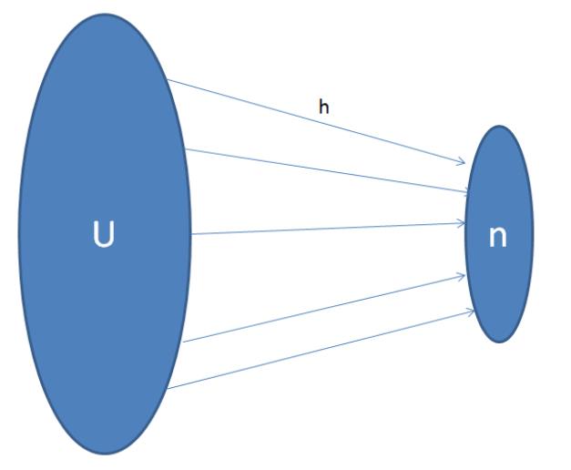
Throughout this section, we consider a family H of hash functions, with each h ∈ H mapping
a large universe U to a relatively small number of “buckets” {1, 2, . . . , n} (Figure 1). We’ll be
thinking about the following experiment, which should be familiar from CS161: an adversary
picks an arbitrary data set S ⊆ U, then we pick a hash function h ∈ H uniformly at random
and use it to hash all of the elements of S. We’d like these objects to be distributed evenly
across the buckets, and the maximum load of a bucket (i.e., the number of items hashing
to it) is a natural measure of distance from this ideal case. For example, in a hash table
with chaining, the maximum load of a bucket governs the worst-case search time, a highly
relevant statistic.
3
.2 Markov’s Inequality
For now, all we assume about H is that each object is equally likely to map to each bucket
(though not necessarily independently).
(P1) For every x ∈ U and i ∈ {1, 2, . . . , n}, Prh∈H[h(x) = i] = .
1
n
This property is already enough to analyze the expected load of a bucket. For simplicity,
suppose that the size |S| of the data set being hashed equals the number of buckets n.
Then, for any bucket i, by linearity of expectation (applied to indicator random variables
for elements getting mapped to i), its expected load is
X
|
S|
Pr[h(x) = i] =
= 1.
(1)
|
{z
}
n
x∈S
=
1/n by (P1)
This is good — the expectations seem to indicate that things are balanced on average. But
can we prove a concentration result, stating that loads are close to these expectations?
The following tail inequality gives a weak bound but applies under minimal assumptions;
it is our second (of 5) essential tools for the analysis of randomized algorithms.
Theorem 3.1 (Markov’s Inequality) If X is a non-negative random variable with finite
expectation, then for every constant c ≥ 1,
1
Pr[X ≥ c · E[X]] ≤ .
c
For example, such a random variable is at least 10 times its expectation at most 10% of the
time, and is at least 100 times its expectation at most 1% of the time. In general, Markov’s
inequality is useful when a constant probability guarantee is good enough. The proof of
Markov’s inequality is easy, and we leave it to Exercise Set #9.3
3
Both hypotheses are necessary. For example, random variables that are equally likely to be M or −M
exhibit no concentration whatsoever as M → ∞.
5


We now apply Markov’s inequality to the random variable equal to the load of our favorite
bucket i. We can choose any c ≥ 1 we want in Theorem 3.1. For example, choosing c = n
and recalling that the relevant expectation is 1 (assuming |S| = n), we obtain
1
Pr[load of i ≥ n] ≤
.
n
1
The good news is that is not a very big number when n is large. But let’s look at the
event we’re talking about: the load of i being at least n means that every single element of
n
S hashes to i. And this sounds crazy, like it should happen much less often than 1/n of the
time. (If you hash 100 things into a hash table with 100 buckets, would you really expect
everything to hash to the same bucket 1% of the time?)
If we’re only assuming the property (P1), however, it’s impossible to prove a better bound.
To see this, consider the set H = {h(x) = i : i = 1, 2, . . . , n} of constant hash functions,
each of which maps all items to the same bucket. Observe that H satisfies property (P1).
1
But the probability that all items hash to the bucket i is indeed .
n
3
.3 Chebyshev’s Inequality
A totally reasonable objection is that the example above is a stupid family of hash function
that no one would ever use. So what about a good family of hash functions, like those you
studied in CS161? Specifically, we now assume:
(P2) for every pair x, y ∈ U of distinct elements, and every i, j ∈ {1, 2, . . . , n},
1
Prh∈H[h(x) = i and h(y) = j] =
.
n2
That is, when looking at only two elements, the joint distribution of their buckets is as if
the function h is a totally random function. (Property (P1) asserts an analogous statement
when looking at only a single element.) A family of hash functions satisfying (P2) is called
a pairwise or 2-wise independent family. This is almost the same as (and for practical
purposes equivalent to) the notion of “universal hashing” that you saw in CS161. The
family of constant hash functions (above) clearly fails to satisfy property (P2).
So how do we use this stronger assumption to prove sharper concentration bounds?
Recall that the variance Var[X] of a random variable is its expected squared deviation from
its mean E[(X − E[X])2], and that the standard deviation is the square root of the variance.
Assumption (P2) buys us control over the variance of the load of a bucket. Chebyshev’s
inequality, the third of our five essential tools, is the inequality you want to use when the
best thing you’ve got going for you is a good bound on the variance of a random variable.
Theorem 3.2 (Chebyshev’s Inequality) If X is a random variable with finite expecta-
tion and variance, then for every constant t ≥ 1,
1
Pr[|X − E[X] | > t · StdDev[X]] ≤
.
t2
6


For example, the probability that a random variable differs from its expectation by at least
two standard deviations is at most 25%, and the probability that it differs by at least 10
standard deviations is at most 1%. Chebyshev’s inequality follows easily from Markov’s
inequality; see Exercise Set #9.
Now let’s go back to the load of our favorite bucket i, where a data set S ⊆ U with size
|
S| = n is hashed using a hash function h chosen uniformly at random from H. Call this
random variable X. We can write
X
X =
Xy,
y∈S
where X is the indicator random variable for whether or not h(y) = i. We noted earlier
y
that, by (P1), E[X] =
P
1
= 1.
Now consider the variance of X. We claim that
y∈S n
X
Var[X] =
Var[Xy] ,
(2)
y∈S
analogous to linearity of expectation. Note that this statement is not true in general — e.g.,
if X and X are indicator random variables of complementary events, then X +X is always
2
1
2
1
equal to 1 and hence has variance 0. In CS109 you saw a proof that for independent random
variables, variances add as in (2). If you go back and look at this derivation — seriously,
go look at it — you’ll see that the variance of a sum equals the sum of the variances of
the summands, plus correction terms that involve the covariances of pairs of summands.
The covariance of independent random variables is zero. Here, we are only dealing with
pairwise independent random variables (by assumption (P2)), but still, this implies that the
covariance of any two summands is 0. We conclude that (2) holds not only for sums of
independent random variables, but also of pairwise independent random variables.
1
Each indicator random variable X is a Bernoulli variable with parameter , and so
1
y
1. Using (2), we have Var[X] =
P
n
= 1. (By
Var[X ] = (1
y
− 1
)
≤
Var[Xy]
≤
n
· 1
n
n
y
∈
S
n
contrast, when H is the set of constant hash functions, Var[X] ≈ n.)
Applying Chebyshev’s inequality with t = n (and ignoring “+1” terms for simplicity),
we obtain
1
Prh∈H[X ≥ n] ≤
.
n2
This is a better bound than what we got from Markov’s inequality, but it still doesn’t seem
that small — when hashing 10 elements into 10 buckets, do you really expect to see all of them
in a single bucket 1% of the time? But again, without assuming more than property (P2),
we can’t do better — there exist families of pairwise independent hash functions such that
1
all elements hash to the same bucket with probability ; showing this is a nice puzzle.
n2
3
.4 Chernoff Bounds
In this section we assume that:
(P3) all h(x)’s are uniformly and independently distributed in {1, 2, . . . , n}. Equivalently,
h is completely random function.
7


How can we use this strong assumption to prove sharper concentration bounds?
The fourth of our five essential tools for analyzing randomized algorithms is the Chernoff
bounds. They are the centerpiece of this lecture, and are used all the time in the analysis of
algorithms (and also complexity theory, machine learning, etc.).
The point of the Chernoff bounds is to prove sharp concentration for sums of independent
and bounded random variables.
Theorem 3.3 (Chernoff Bounds) Let X , . . . , X be random variables, defined on the
1
same state space and taking values in [0, 1], and set X =
n
P
n
j=1
Xj. Then:
(i) for every δ > 0,
ꢀ
ꢁ
(1+δ)E[X]
e
Pr[X > (1 + δ)E[X]] <
.
1
+ δ
(ii) for every δ ∈ (0, 1),
Pr[X < (1 − δ)E[X]] < e−δ2E[X]/2.
The key thing to notice in Theorem 3.3 is that the deviation probability decays exponentially
in both the factor of the deviation (1+δ) and the expectation of the random variable (E[X]).
So if either of these quantities is even modestly big, then the deviation probability is going
to be very small.4
We could prove Theorem 3.3 in 30 minutes or less, but the right place to spend time
on the proof is a randomized algorithms class (like CS265). So we’ll just use the Chernoff
bounds as a “black box” — this is how almost everybody thinks about them, anyways. It’s
notable that, of our five essential tools for the analysis of randomized algorithms, only the
Chernoff bounds require a non-trivial proof. We’ll only use part (i) in this lecture, but (ii)
is also useful in many situations. An analog of Theorem 3.3 for random variables that are
nonnegative and bounded (not necessarily in [0, 1]) follows from a simple scaling argument.
The independence assumption can be relaxed, for example to negatively correlated random
variables, although the proof then requires a bit more work.
Now let’s apply the Chernoff bounds to analyze the number of items hashing to our
favorite bucket i, under the assumption (P3) that h is a uniformly random function. Again
using X to denote the indicator random variable for the event that h(y) = i, we see that
Py
X =
Xy is now the sum of independent 0-1 random variables, and hence is right in
y∈S
the wheelhouse of the Chernoff bounds. For example, setting 1 + δ = ln n and recalling that
E[X] = 1, Theorem 3.3 implies that
ꢂ
. More generally, a constant less than one
ꢃ
e
ln n
Pr[X > ln n] <
.
(3)
ln n
1
ln n
1
To interpret this bound, note that ( )
raised to a logarithmic power yields an inverse polynomial. Now
=
e
n
e
ln n
is smaller than any
4
For the first bound (i), it is common to state the tighter probability upper bound of [eδ/(1+δ)(1+δ)]E[X],
but the simpler bound here suffices for almost all applications.
8


constant as n grows large, and hence the probability bound in (3) is smaller than any inverse
polynomial. Notice how much better this is than what we could prove using Markov’s or
Chebyshev’s inequality — we’re looking at a much smaller deviation (ln n instead of n) yet
obtaining a much smaller probability bound (smaller than any inverse polynomial).
Theorem 3.3 even implies that
ꢄ
ꢅ
3
ln n
1
Pr X >
≤
,
(4)
ln ln n
n2
as you should verify. Why ln n/ ln ln n? Because this is roughly the solution to the equation
xx = n (this is relevant in Theorem 3.3 because of the (1 + δ)−(1+δ) term). Again, this is a
huge improvement over what we obtained using Markov’s and Chebyshev’s inequalities. For
a more direct comparison, note that Chernoff bounds imply that the probability Pr[X ≥ n] is
at most an inverse exponential function of n (as opposed to an inverse polynomial function).
3
.5 The Union Bound
Figure 2: Area of union is bounded by sum of areas of the circles.
Our fifth essential analysis tool is the union bound, which is not a tail inequality but is
often used in conjunction with tail inequalities. The union bound just says that for events
E , . . . , E ,
1
k
Xk
Pr[at least once of Ei occurs] ≤
Pr[Ei] .
i=1
Importantly, the events are completely arbitrary, and do not need to be independent. The
proof is a one-liner. In terms of Figure 2, the union bound just says that the area (i.e.,
probability mass) in the union is bounded above by the sum of the areas of the circles.
The bound is tight if the events are disjoint; otherwise the right-hand side is larger, due to
double-counting. (It’s like inclusion-exclusion, but without any of the correction terms.) In
9


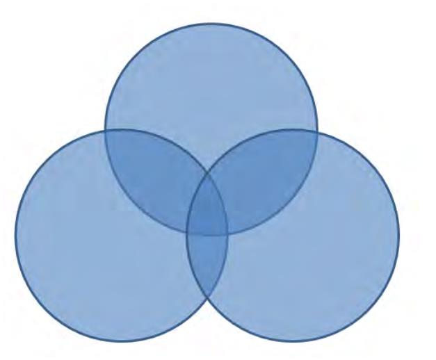
applications, the events E , . . . , E are often “bad events” that we’re hoping don’t happen;
1
k
the union bound says that as long as each event occurs with low probability and there aren’t
too many events, then with high probability none of them occur.
Returning to our running hashing example, let Ei denote the event that bucket i receives
a load larger than 3 ln n/ ln ln n. Using (4) and the union bound, we conclude that with
probability at least 1 − , none of the buckets receive a load larger than 3 ln n/ ln ln n. That
1
n
is, the maximum load is O(log n/ log log n) with high probability.5
3
.6 Chernoff Bounds: The Large Expectation Regime
We previously noted that the Chernoff bounds yield very good probability bounds once the
deviation (1+δ) or the expectation (E[X]) becomes large. In our hashing application above,
we were in the former regime. To illustrate the latter regime, suppose that we hash a data
set S ⊆ U with |S| = n ln n (instead of ln n). Now, the expected load of every bucket is ln n.
Applying Theorem 3.3 with 1 + δ = 4, we get that, for each bucket i,
ꢂ ꢃ
e
4 ln n
1
Pr[load on i is > 4 ln n] ≤
≤
.
4
n2
Using the union bound as before, we conclude that with high probability, no bucket receives
a load more than a small constant factor times its expectation.
Summarizing, when loads are light there can be non-trivial deviations from expected
loads (though still only logarithmic). Once loads are even modestly larger, however, the
buckets are quite evenly balanced with high probability. This is a useful lesson to remember,
for example in load-balancing applications (in data centers, etc.).
4
Randomized Rounding
We now return to the design and analysis of approximation algorithms, and give a classic
application of the Chernoff bounds to the problem of low-congestion routing.
Figure 3: Example of edge-disjoint path problem. Note that vertices can be shared, as shown
in this example.
5
There is also a matching lower bound (up to constant factors).
1
0


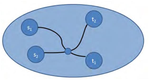

If the edge-disjoint paths problems, the input is a graph G = (V, E) (directed or undi-
rected) and source-sink pairs (s , t ), . . . , (s , t ). The goal is to determine whether or not
1
there is an s -t path P for each i such that no edge appears in more than one of the P ’s.
1
k
k
i
i
i
i
See Figure 3. The problem is NP-hard (for directed graphs, even when k = 2).
Recall from last lecture the linear programming rounding approach to approximation
algorithms:
1
. Solve an LP relaxation of the problem. (For an NP-hard problem, we expect the
optimal solution to be fractional, and hence not immediately meaningful.)
2
. “Round” the resulting fractional solution to a feasible (integral) solution, hopefully
without degrading the objective function value by too much.
Last lecture applied LP rounding to the vertex cover problem. For the edge-disjoint paths
problem, we’ll use randomized LP rounding. The idea is to interpret the fractional values
in an LP solution as specifying a probability distribution, and then to round variables to
integers randomly according to this distribution.
The first step of the algorithm is to solve the natural linear programming relaxation of
the edge-disjoint paths problem. This is just a multicommodity flow problem (as in Exercise
Set #5 and Problem Set #3). In this relaxation the question is whether or not it is possible
to send simultaneously one unit of (fractional) flow from each source si to the corresponding
sink ti, where every edge has a capacity of 1. 0-1 solutions to this multicommodity flow
problem correspond to edge-disjoint paths. As we’ve seen, this LP relaxation can be solved
in polynomial time. If this LP relaxation is infeasible, then we can conclude that the original
edge-disjoint paths problem is infeasible as well.
Assume now that the LP relaxation is feasible. The second step rounds each s -t pair
i
i
independently. Consider a path decomposition (Problem Set #1) of the flow being pushed
from s to t . This gives a collection of paths, together with some amount of flow on each
i
path. Since exactly one unit of flow is sent, we can interpret this path decomposition as
i
a probability distribution over s -t paths. The algorithm then just selects an s -t path
i
i
randomly according to this probability distribution.
i
i
The rounding step yields paths P , . . . , P . In general, they will not be disjoint (this
1
k
would solve an NP-hard problem), and the goal is to prove that they are approximately
disjoint in some sense. The following result is the original and still canonical application of
randomized rounding.
Theorem 4.1 Assume that the LP relaxation is feasible. Then with high probability, the
randomized rounding algorithm above outputs a collection of paths such that no edge is used
by more than
3
ln m
ln ln m
of the paths, where m is the number of edges.
The outline of the proof is:
1
1

1
2
. Fix an edge e. The expected number of paths that include e is at most 1. (By linearity
of expectation, it is precisely the amount of flow sent on e by the multicommodity flow
relaxation, which is at most 1 since all edges were given unit capacity.)
. Like in the hashing analysis in Section 3.6,
ꢄ
ꢅ
3
ln m
1
Pr # paths on e >
≤
,
ln ln m
m2
where m is the number of edges. (Edges are playing the role of buckets, and s -t pairs
i
i
as items.)
1
m
3
. Taking a union bound over the m edges, we conclude that with all but probability,
every edge winds up with at most 3 ln m/ ln ln m paths using it.
Zillions of analyses in algorithms (and theoretical computer science more broadly) use this
one-two punch of the Chernoff bound and the union bound.
Interestingly, for directed graphs, the approximation guarantee in Theorem 4.1 is optimal,
up to a constant factor (assuming P = NP). For undirected graphs, there is an intriguing
gap between the O(log n/ log log n) upper bound of Theorem 4.1 and the best-know lower
bound of Ω(log log n) (assuming P = NP).
5
Epilogue
To recap the top 5 essential tools for the analysis of randomized algorithms:
1
2
3
4
. Linearity of expectation. If all you care about is the expectation of a random variable,
this is often good enough.
. Markov’s inequality. This inequality usually suffices if you’re satisfied with a constant-
probability bound.
. Chebyshev’s inequality. This inequality is the appropriate one when you have a good
handle on the variance of your random variable.
. Chernoff bounds. This inequality gives sharp concentration bounds for random vari-
ables that are sums of independent and bounded random variables (most commonly,
sums of independent indicator random variables).
5
. Union bound. This inequality allows you to avoid lots of bad low-probability events.
All five of these tools are insanely useful. And four out of the five have one-line proofs!
1
2


CS261: A Second Course in Algorithms
Lecture #19: Beating Brute-Force Search∗
Tim Roughgarden†
March 8, 2016
A popular myth is that, for NP-hard problems, there are no algorithms with worst-case
running time better than that of brute-force search. Reality is more nuanced, and for many
natural NP-hard problems, there are algorithms with (worst-case) running time much better
than the naive brute-force algorithm (albeit still exponential). This lecture proves this point
by revisiting three problems studied in previous lectures: vertex cover, the traveling salesman
problem, and 3-SAT.
1
Vertex Cover and Fixed-Parameter Tractability
This section studies the special case of the vertex cover problem (Lecture #18) in which
every vertex has unit weight. That is, given an undirected graph G = (V, E), the goal is to
compute a minimum-cardinality subset S ⊆ V that contains at least one endpoint of every
edge.
We study the problem of checking whether or not a vertex cover instance admits a vertex
cover of size at most k (for a given k). This problem is no easier than the general problem,
since the latter reduces to the former by trying all possible values of k. Here, you should
think of k as “small,” for example between 10 and 20. The graph G can be arbitrarily
large, but think of the number of vertices as somewhere between 100 and 1000. We’ll show
how to beat brute-force search for small k. This will be our only glimpse of “parameterized
algorithms and complexity,” which is a vibrant subfield of theoretical computer science.
The naive brute-force search algorithm for checking whether or not there is a vertex cover
of size at most k is: for every subset S ⊆ V of k vertices, check whether or not S is a vertex
ꢀ
ꢁ
n
k
k
cover. The running time of this algorithm scales as
, which is Θ(n ) when k is small.
While technically polynomial for any constant k, there is no hope of running this algorithm
unless k is extremely small (like 3 or 4).
If we aim to do better, what can we hope for? Better than Θ(nk) would a running time
of the form poly(n) · f(k), where the dependence on k and on n can be separated, with
∗
†
ꢀc
2
Department of Computer Science, Stanford University, 474 Gates Building, 353 Serra Mall, Stanford,
016, Tim Roughgarden.
CA 94305. Email: tim@cs.stanford.edu.
1

the latter dependence only polynomial. Even better would be a running time of the form
poly(n) + f(k) for some function k. Of course, we’d like the poly(n) term to be as close to
linear as possible. We’d also like the function f(k) to be as small as possible, but because
the vertex cover problem is NP-hard for general k, we expect f(k) to be at least exponential
in k. An algorithm with such a running time is called fixed-parameter tractable (FPT) with
respect to the parameter k.
We claim that the following is an FPT algorithm for the minimum-cardinality vertex
cover problem (with budget k).
FPT Algorithm for Vertex Cover
set S = {v ∈ V : deg(v) ≥ k + 1}
set G = G S
\
0
0
0
0
set G equal to G with all isolated vertices removed
0
0
2
if G has more than k edges then
return “no vertex cover with size ≤ k”
else
0
0
compute a minimum-size vertex cover T of G by brute-force search
return “yes” if and only if |S| + |T| ≤ k
We next explain why the algorithm is correct. First, notice that if G has a set cover S
of size at most k, then every vertex with degree at least k + 1 must be in S. For if such a
vertex v is not in S, then the other endpoint of each of the (at least k + 1) edges incident
to v must be in the vertex cover; but then |S| ≥ k + 1. In the second step, G is obtained
0
from G by deleting S and all edges incident to a vertex in S. The edges that survive in G0
are precisely the edges not already covered by S. Thus, the vertex covers of size at most k
in G are precisely the sets of the form S ∪ T, where T is a vertex cover of G size at most
0
k −|S|. Given that every vertex cover with size at most k contains the set S, there is no loss
0
in discarding the isolated vertices of G (all incident edges of such a vertex in G are already
covered by vertices in S). Thus, G has a vertex cover of size at most k if and only if G has
0
0
a vertex cover of size at most k − |S|. In the fourth step, if G has more than k edges, then
0
0
2
it cannot possibly have a vertex cover of size at most k (let alone k − |S|). The reason is
0
that every vertex of G has degree at most k (all higher-degree vertices were placed in S),
so each vertex of G can only cover k edges, so G has a vertex cover of size at most k only
0
0
0
00
if it has at most k2 edges. The final step computes the minimum-size vertex cover of G by
brute force, and so is clearly correct.
Next, observe that in the final step (if reached), the graph G has at most k edges (by
00
0
0
2
assumption) and hence at most 2k2 vertices (since every vertex of G has degree at least 1).
It follows that the brute-force search step can be implemented in 2O(k2) time. Steps 1–4 can
00
be implemented in linear time, so the overall running time is O(m) + 2O(k , and hence the
2
)
0
0
algorithm is fixed-parameter tractable. In FPT jargon, the graph G is called a kernel (of
size O(k2)), meaning that the original problem (on an arbitrarily large graph, with a given
budget k) reduces to the same problem on a graph whose size depends only on k. Using
2

linear programming techniques, it is possible to show that every unweighted vertex cover
instance actually admits a kernel with size only O(k), leading to a running time dependence
on k of 2O(k) rather than 2O(k . Such singly-exponential dependence is pretty much the
best-case scenario in fixed-parameter tractability.
2
)
Just as some problems admit good approximation algorithms and others do not (assuming
P = NP), some problems (and parameters) admit fixed-parameter tractable algorithms
while others do not (under appropriate complexity assumptions). This is made precise
primarily via the theory of “W[1]-hardness,” which parallels the familiar theory of NP-
hardness. For example, the independent set problem, despite its close similarity to the
vertex cover problem (the complement of a vertex cover is an independent set and vice
versa), is W[1]-hard and hence does not seem to admit a fixed-parameter tractable algorithm
(parameterized by the size of the largest independent set).
2
TSP and Dynamic Programming
Recall from Lecture #16 the traveling salesman problem (TSP): the input is a complete
undirected graph with non-negative edge weights, and the goal to compute the minimum-
cost TSP tour, meaning a simple cycle that visits every vertex exactly once. We saw in
Lecture #16 that the TSP problem is hard to even approximate, and for this reason we
focused on approximation algorithms for the (still NP-hard) special case of the metric TSP.
Here, we’ll give an exact algorithm for TSP, and we won’t even assume that the edges satisfy
the triangle inequality.
The naive brute-force search algorithm for TSP tries every possible tour, leading to
a running time of roughly n!, where n is the number of vertices. Recall that n! grows
considerably faster than any function of the form cn for a constant c (see also Section 3).
Naive brute-force search is feasible with modern computers only for n in the range of 12
or 13. This section gives a dynamic programming algorithm for TSP that runs in O(n22n)
time. This extends the “tractability frontier” for n into the 20s. One drawback of the
dynamic programming algorithm is that it also uses exponential space (unlike brute-force
search). It is an open question whether or not there is an exact algorithm for TSP that has
running time O(cn) for a constant c > 1 and also uses only a polynomial amount of space.
Two take-aways from the following algorithm are: (i) TSP is another fundamental NP-hard
problem for which algorithmic ingenuity beats brute-force search; and (ii) your algorithmic
toolbox (here, dynamic programming) continues to be extremely useful for the design of
exact algorithms for NP-hard problems.
Like any dynamic programming algorithm, the plan is to solve systematically a collection
of subproblems, from “smallest” to “largest,” and then read off the final answer from the
biggest subproblems. Coming up with right subproblems is usually the hardest part of
designing a dynamic programming algorithm. Here, in the interests of time, we’ll just cut
to the chase and state the relevant subproblems.
Let V = {1, 2, . . . , n} be the vertex set. The algorithm populates a two-dimensional
array A, with one dimension indexed by a subset S ⊆ V of vertices and the other dimension
3
indexed by a single vertex j. At the end of the algorithm, the entry A[S, j] will contain the
cost of the minimum-cost path that:
(i) visits every vertex v ∈ S exactly once (and no other vertices);
(ii) starts at the vertex 1 (so 1 better be in S);
(iii) ends at the vertex j (so j better be in S).
There are O(n2n) subproblems. Since the TSP is NP-hard, we should not be surprised to
see an exponential number of subproblems.
After solving all of the subproblems, it is easy to compute the cost of an optimal tour
in linear time. Since A[{1, 2, . . . , n}, j] contains the length of the shortest path from 1 to j
that visits every vertex exactly once, we can just “guess” (i.e., do brute-force search over)
the vertex preceding 1 on the tour:
n
OPT = min A[{1, 2, . . . , n}, j] + c .
j1
{
z
}
|{z}
j=2
|
path from 1 to j
last hop
Next, we need a principled way to solve all of the subproblems, using solutions to pre-
viously solved “smaller” subproblems to quickly solve “larger” subproblems. That is, we
need a recurrence relating the solutions of different subproblems. So consider a subproblem
A[S, j], where the goal is to compute the minimum cost of a path subject to (i)–(iii) above.
What must the optimal solution look like? If we only knew the penultimate vertex k on the
path (right before j), then we would know what the path looks like: it would be the cheapest
possible path visiting each of the vertices of S \ {j} exactly once, starting at 1, and ending
at k (why?), followed of course by the final hop from k to j. Our recurrence just executes
brute-force search over all of the legitimate choices of k:
A[S, j] = k∈mS\i{n1,j} (A[S \ {j}, k] + ckj) .
This recurrence assumes that |S| ≥ 3. If |S| = 1 then A[S, j] is 0 if S = {1} and j = 1 and
is +∞ otherwise. If |S| = 2, then the only legitimate choice of k is 1.
The algorithm first solves all subproblems with |S| = 1, then all subproblems with
|
S| = 2, . . . , and finally all subproblems with |S| = n (i.e., S = {1, 2, . . . , n}). When solving
a subproblem, the solutions to all relevant smaller subproblems are available for constant-
time lookup. Each subproblem can thus be solved in O(n) time. Since there are O(n2n)
subproblems, we obtain the claimed running time bound of O(n22n).
3
3SAT and Random Search
3
.1 Scho¨ning’s Algorithm
Recall from last lecture that a 3SAT formula involves n Boolean variables x , . . . , x and m
1
clauses, where each clause is the disjunction of three literals (where a literal is a variable or
n
4


its negation). Last lecture we studied MAX 3SAT, the optimization problem of satisfying as
many of the clauses as possible. Here, we’ll study the simpler decision problem, where the
goal is to check whether or not there is a assignment that satisfies all m clauses. Recall that
this is the canonical example of an NP-complete problem (cf., the Cook-Levin theorem).
Naive brute-force search would try all 2n truth assignments. Can we do better than
exhaustive search? Intriguingly, we can, with a simple algorithm and by a pretty wide
margin. Specifically, we’ll study Sch¨oning’s random search algorithm (from 1999). The
parameter T will be determined later.
Random Search Algorithm for 3SAT (Version 1)
repeat T times (or until a satisfying assignment is found):
choose a truth assignment a uniformly at random
repeat n times (or until a satisfying assignment is found):
choose a clause C violated by the current assignment a
choose one the three literals from C uniformly at random, and
modify a by flipping the value of the corresponding variable
(from “true” to “false” or vice versa)
if a satisfying assignment was found then
return “satisfiable”
else
return “unsatisfiable”
And that’s it!1
3
.2 Analysis (Version 1)
We give three analyses of Scho¨ning’s algorithm (and a minor variant), each a bit more so-
phisticated and establishing a better running time bound than the last. The first observation
is that the algorithm never makes a mistake when the formula is unsatisfiable — it will never
find a satisfying assignment (no matter what its coin flips are), and hence reports “unsatis-
fiable.” So what we’re worried about is the algorithm failing to find a satisfying assignment
when one exists. So for the rest of the lecture, we consider only satisfiable instances. We
use a∗ to denote a reference satisfying assignment (if there are many, we pick one arbitrar-
ily). The high-level idea is to track the “Hamming distance” between a∗ and our current
truth assignment a (i.e., the number of variables with different values in a and a∗). If this
Hamming distance ever drops to 0, then a = a∗ and the algorithm has found a satisfying
assignment.
1
A little backstory: an analogous algorithm for 2SAT (2 literals per clause) was studied earlier by Pa-
padimitriou. 2SAT is polynomial-time solvable — for example, it can be solved in linear time via a reduction
to computing the strongly connected components of a suitable directed graph. Papadimitriou’s random search
algorithm is slower but still polynomial (O(n2)), with the analysis being a nice exercise in random walks
(covered in the instructor’s Coursera videos).
5


A simple observation is that, if the current assignment a fails to satisfy a clause C, then
∗
∗
a assigns at least one of the three variables in C a different value than a does (as a satisfies
the clause). Thus, when the random search algorithm chooses a variable of a violated clause
to flip, there is at least a 1/3 chance that the algorithm chooses a “good variable,” the
flipping of which decreases the Hamming distance between a and a∗ by one. (If a and a∗
differ on more than one variable of C, then the probability is higher.) In the other case,
when the algorithm chooses a “bad variable,” where a and a∗ give it the same value, flipping
the value of the variable in a increases the Hamming distance between a and a∗ by 1. This
happens with probability at most 2/3.2
All of the analyses proceed by identifying simple sufficient conditions for the random
search algorithm to find a satisfying assignment, bounding below the probability that these
sufficient conditions are met, and then choosing T large enough that the algorithm is guar-
anteed to succeed with high probability.
To begin, suppose that the initial random assignment a chosen in an iteration of the outer
loop differs from the reference satisfying assignment a∗ in k variables. A sufficient condition
for the algorithm to succeed is that, in every one of the first k iterations of the inner loop, the
algorithm gets lucky and flips the value of a variable on which a, a∗ differ. Since each inner
loop iteration has a probability of at least 1/3 of choosing wisely, and the random choices
are independent, this sufficient condition for correctness holds with probability at least 3 .
k
−
(The algorithm might stop early if it stumbles on a satisfying assignment other than a∗; this
is obviously fine with us.)
For our first analysis, we’ll use a sloppy argument to analyze the parameter k (the distance
between a and a∗ at the beginning of an outer loop iteration). By symmetry, a agrees with a∗
on at least half the variables (i.e., k ≤ n/2) with probability at least 1/2. Conditioning on this
event, we conclude that a single outer loop iteration successfully finds a satisfying assignment
1
with probability at least p =
. Hence, the algorithm finds a satisfying assignment in one
2
·3n/2
of the T outer loop iterations except with probability at most (1 − p)T ≤ e . If we take
−
pT 3
d ln n
T =
for a constant d > 0, then the algorithm succeeds except with inverse polynomial
1
p
probability . Substituting for p, we conclude that
nd
ꢂ
ꢃ
√
T = Θ ( 3) log n
n
outer loop iterations are enough to be correct with high probability. This gives us an al-
gorithm with running time O((1.74)n), which is already significantly better than the 2n
dependence in brute-force search.
2
The fact that the random process is biased toward moving farther away from a∗ is what gives rise to
the exponential running time. In the case of 2SAT, each random move is at least as likely to decrease the
distance as increase the distance, which in turn leads to a polynomial running time.
Recall the useful inequality 1 + x ≤ ex for all x ∈ R, used also in Lectures #11 (see the plot there) and
3
#
15.
6


3
.3 Analysis (Version 2)
We next give a refined analysis of the same algorithm. The plan is to count the probability
of success for all values of the initial distance k, not just when k ≤ n/2 (and not assuming
the worst case of k = n/2).
For a given choice of k ∈ {1, 2, . . . , n}, what is the probability that the initial assignment
∗
a and a differ in their values to exactly k variables? There is one such assignment for each
ꢀ
ꢁ
n
of the
with a on S and disagrees with a outside of S.) Since all truth assignments are equally
choices of a set S of k out of n variables. (The corresponding assignment a agrees
k
∗
likely (probability 2 each),
∗
−
n
ꢄ ꢅ
n
k
Pr[dist(a, a∗) = k] =
−n
2 .
We can now lower bound the probability of success of an outer loop iteration by condi-
tioning on k:
Xn
∗
∗
Pr[success] =
Pr[dist(a, a ) = k] · E[success | dist(a, a ) = k]
k=0
Xn
ꢄ ꢅ
ꢄ ꢅ
k
n
k
1
3
2−
n
≥
k=0
−
n
1
n
=
=
2 (1 + )
3
ꢄ ꢅ
n
2
3
,
where the penultimate equality follows from a slick application of the binomial formula.4
Thus, taking T = Θ(( ) log n), the random search algorithm is correct with high prob-
n
3
2
ability.
3
.4 Analysis (Version 3)
For the final analysis, we tweak the version of Scho¨ning’s algorithm above slightly, replacing
repeat n times” in the inner loop by “repeat 3n times.” This only increases the running
“
time by a constant factor.
Our two previous analyses only considered the cases where the random search algorithm
made a beeline for the reference satisfying assignment a∗, never making an incorrect choice
of which variable to flip. There are also other cases where the algorithm will succeed.
For example, if the algorithm chooses a bad variable once (increasing dist(a, a∗) by 1),
but then a good variable k + 1 times, then after these k + 2 iterations a is the same as
the satisfying assignment a∗ (unless the algorithm stopped early due to finding a different
satisfying assignment).
P
ꢀ ꢁ
4
I.e., the formula (a + b)n =
n
k=0
n akbn−k.
k
7


For the analysis, we’ll focus on the specific case where, in the first 3k inner loop iterations,
the algorithm chooses a bad variable k times and a good variable 2k times. This idea leads
to
ꢄ ꢅꢄ ꢅ ꢄ ꢅ ꢄ ꢅ
Xn
2k
k
n
k
3k
1
3
2
3
n
Pr[success] ≥
2−
,
(1)
k
k=0
since the probability that the random local search algorithm chooses a good variable 2k
3
ꢀ
ꢁ
k
k
( ) ( ) .
2k
1
3
2
3
k
times in the first 3k inner loop iterations is at least
This inequality is pretty messy, with no less than two binomial coefficients complicating
ꢀ
ꢁ
n
each summand. We’ll be able to handle the
terms using the same slick binomial expansion
terms are more annoying. To deal with them,
ꢀ
kꢁ
3
k
trick from the previous analysis, but the
recall Stirling’s approximation for the factorial function:
k
ꢂ
ꢂ ꢃ ꢃ
√
n
e
n
n! = Θ
n
.
√
(The hidden constant is 2π, but we won’t need to worry about that.) Thus, in the grand
scheme of things, n! is not all that much smaller than nn.
ꢀ
ꢁ
3
k
k
We can use Stirling’s approximation to simplify
:
ꢄ ꢅ
3
k
(3k!)
=
=
=
k
(2k)!k!
ꢄ
!
√
3
e
k
3k
3
k
( )
Θ
√ √
·
ꢅ
k
k
2k 2k
e
k 2k ( ) ( )
e
1
33k
Θ √ ·
.
2
2k
k
Thus,
ꢄ ꢅ ꢄ ꢅ ꢄ ꢅ
ꢄ
ꢅ
2
k
k
−
2
k
3
k
1
3
2
3
=
Θ √
.
k
k
|
{z }
√
=
Θ(33k/22k k)
8


Substituting back into (1), we find that for some constant c > 0 (hidden in the Θ notation),
ꢄ ꢅꢄ ꢅ ꢄ ꢅ ꢄ ꢅ
Xn
k=0
c2−
2k
k
n
3k
1
3
2
3
n
Pr[success] ≥
2−
k
k
ꢄ ꢅ
Xn
−
k
n 2
n
√
≥
≥
k
k
k=0
ꢄ ꢅ
Xn
c
n
k
−
n
2−k
√ 2
n
k=0
ꢄ
ꢅ
n
c
1
−
n
=
=
√ 2
1 +
n
2
ꢄ ꢅ
n
c
3
4
√
.
n
ꢀ
ꢀ ꢁ √
ꢁ
n
4
3
n
We conclude that with T = Θ
n log n , the algorithm is correct with high probability.
This running time of ≈ ( ) has been improved somewhat since 1999, but this is still
4
3
quite close to the state of the art, and it is an impressive improvement over the ≈ 2n running
time require by brute-force search. Can we do even better? This is an open question.
The exponential time hypothesis (ETH) asserts that every correct algorithm for 3SAT has
worst-case running time at least cn for some constant c > 1. (For example, this rules out a
“
quasi-polynomial-time” algorithm, with running time npolylog(n).) The ETH is certainly a
stronger assumption than P = NP, but most experts believe that it is true.
The random search idea can be extended from 3SAT to k-SAT for all constant values
of k. For every constant k, the result is an algorithm that runs in time O(cn) for a constant
c < 2. However, the constant c tends to 2 as k tends to infinity. The strong exponential
time hypothesis (SETH) asserts that this is necessary — that there is no algorithm for the
general SAT problem (with k arbitrary) that runs in worst-case running time O(cn) for some
constant c < 2 (independent of k). Expert opinion is mixed on whether or not SETH holds.
If it does hold, then there are interesting consequences for lots of different problems, ranging
from the prospects of fixed-parameter tractable algorithms for NP-hard problems (Section 1)
to lower bounds for classic algorithmic problems like computing the edit distance between
two strings.
9


CS261: A Second Course in Algorithms
Lecture #20: The Maximum Cut Problem and
Semidefinite Programming∗
Tim Roughgarden†
March 10, 2016
1
Introduction
Now that you’re finishing CS261, you’re well equipped to comprehend a lot of advanced
material on algorithms. This lecture illustrates this point by teaching you about a cool and
famous approximation algorithm.
In the maximum cut problem, the input is an undirected graph G = (V, E) with a
nonnegative weight w ≥ 0 for each edge e ∈ E. The goal is to compute a cut — a partition
e
of the vertex set into sets A and B — that maximizes the total weight of the cut edges (the
edges with one endpoint in each of A and B).
Now, if it were the minimum cut problem, we’d know what to do — that problem reduces
to the maximum flow problem (Exercise Set #2). It’s tempting to think that we can reduce
the maximum cut problem to the minimum cut problem just by negating the weights of all
of the edges. Such a reduction would yield a minimum cut problem with negative weights
(or capacities). But if you look back at our polynomial-time algorithms for computing
minimum cuts, you’ll notice that we assumed nonnegative edge capacities, and that our
proofs depended on this assumption. Indeed, it’s not hard to prove that the maximum cut
problem is NP-hard. So, let’s talk about polynomial-time approximation algorithms.
1
It’s easy to come up with a -approximation algorithm for the maximum cut problem.
Almost anything works — a greedy algorithm, local search, picking a random cut, linear pro-
2
gramming rounding, and so on. But frustratingly, none of these techniques seemed capable
1
of proving an approximation factor better than . This made it remarkable when, in 1994,
Goemans and Williamson showed how a new technique, “semidefinite programming round-
2
ing,” could be used to blow away all previous approximation algorithms for the maximum
cut problem.
∗
†
ꢀc
2
Department of Computer Science, Stanford University, 474 Gates Building, 353 Serra Mall, Stanford,
016, Tim Roughgarden.
CA 94305. Email: tim@cs.stanford.edu.
1


2
A Semidefinite Programming Relaxation for the Max-
imum Cut Problem
2
.1 A Quadratic Programming Formulation
To motivate a novel relaxation for the maximum cut problem, we first reformulate the
problem exactly via a quadratic program. (So solving this program is also NP-hard.) The
idea is to have one decision variable y for each vertex i ∈ V , indicating which side of the
i
cut the vertex is on. It’s convenient to restrict y to lie in {−1, +1}, as opposed to {0, 1}.
i
There’s no need for any other constraints. In the objective function, we want an edge (i, j)
of the input graph G = (V, E) to contribute wij whenever i, j are on different sides of the
cut, and 0 if they are on the same side of the cut. Note that y y = +1 if i, j are on the
i
j
same side of the cut and y y = −1 otherwise. Thus, we can formulate the maximum cut
i
objective function exactly as
j
X
1
max
w · (1 − y y ) .
ij
i
j
2
(i,j)∈E
Note that the contribution of edge (i, j) to the objective function is wij if i and j are on
different sides of the cut and 0 otherwise, as desired. There is a one-to-one and objective-
function-preserving correspondence between cuts of the input graph and feasible solutions
to this quadratic program.
This quadratic programming formulation has two features that make it a non-linear
program: the integer constraints y ∈ {±1} for every i ∈ V , and the quadratic terms y y in
i
i
j
the objective function.
2
.2 A Vector Relaxation
Here’s an inspired idea for a relaxation: rather than requiring each yi to be either -1 or +1,
we only ask that each decision variable is a unit vector in Rn, where n = |V | denotes the
number of vertices. We henceforth use x to denote the (vector-valued) decision variable
i
corresponding to the vertex i ∈ V . We can think of the values +1 and -1 as the special cases
of the unit vectors (1, 0, 0, . . . , 0) and (−1, 0, 0, . . . , 0). There is an obvious question of what
we mean by the quadratic term y y˙ when we switch to decision variables that are n-vectors;
i
j
the most natural answer is to replace the scalar product y · y by the inner product hx , x i.
i
We then have the following “vector programming relaxation” of the maximum cut problem:
j
i
j
X
1
2
max
w (1 − hx , x i)
ij
i
j
(i,j)∈E
subject to
2
2
kx k = 1
for every i ∈ V .
i
It may seem obscure to write kx k2 = 1 rather than kx k2 = 1 (which is equivalent); the
i
reason for this will become clear later in the lecture. Since every cut of the input graph G
2
i
2
2


maps to a feasible solution of this relaxation with the same objective function value, and the
vector program only maximizes over more stuff, we have
vector OPT ≥ OP T.
Geometrically, this relaxation maps all the vertices of the input graph G to the unit
sphere in Rn, while attempting to map the endpoints of each edge to points that are as close
to antipodal as possible (to get hx , x i as close to -1 as possible).
i
j
2
.3 Disguised Convexity
Figure 1: (a) a circle is convex, but (b) is not convex;the chord shown is not contained
entirely in the set.
It turns out that the relaxation above can be solved to optimality in polynomial time.1 You
might well find this counterintuitive, given that the inner products in the objective function
seem hopelessly quadratic. The moral reason for computational tractability is convexity.
Indeed, a good rule of thumb very generally is to equate computational tractability with
convexity. A mathematical program can be convex in two senses. The first sense is the same
as that we discussed back in Lecture #9 — a subset of Rn is convex if it contains all of its
chords. (See Figure 1.) Recall that the feasible region of a linear program is always convex
in this sense. The second sense is that the objective function can be a convex function. (A
linear function is a special case of a convex function.) We won’t need this second type of
convexity in this lecture, but it’s extremely useful in other contexts, especially in machine
learning.
OK. . . but where’s the convexity in the vector relaxation above? After all, if you take the
average of two points on the unit sphere, you don’t get another point on the unit sphere.
We next expose the disguised convexity. A natural idea to remove the quadratic (inner
product) character of the vector program above is to linearize it, meaning to introduce a
new decision variable p for each i, j ∈ V , with the intention that p will take on the value
ij
ij
hx , x i. But without further constraints, this will lead to a relaxation of the relaxation —
i
j
1
Strictly speaking, since the optimal solution might be irrational, we only solve it up to arbitrarily small
error.
3


nothing is enforcing the p ’s to actually be of the form hx , x i for some collection x , . . . , x
ij
of n-vectors, and the p ’s could form an arbitrary matrix instead. So how can we enforce
i
j
1
n
ij
the intended semantics?
This is where elementary linear algebra comes to the rescue. We’ll use some facts that
you’ve almost surely seen in a previous course, and also have almost surely forgotten. That’s
OK — if you spend 20-30 minutes with your favorite linear algebra textbook (or Wikipedia),
you’ll remember why all of these relevant facts are true (none are difficult).
First, let’s observe that a V × V matrix P = {p } is of the form p = hx , x i for some
ij
ij
i
j
vectors x , . . . , x (for every i, j ∈ V ) if and only if we can write
1
n
P = XT X
(1)
for some matrix X ∈ RV . Recalling the definition of matrix multiplication, the (i, j) entry
of XT X is the inner product of the ith row of XT and the jth column of X, or equivalently
the inner product of the ith and jth columns of X. Thus, for matrices P of the desired form,
the columns of the matrix X provide the n-vectors whose inner products define all of the
entries of P.
×
V
Matrices that are “squares” in the sense of (1) are extremely well understood, and they are
called (symmetric) positive semidefinite (psd) matrices. There are many characterizations of
symmetric psd matrices, and none are particularly hard to prove. For example, a symmetric
matrix is psd if and only if all of its eigenvalues are nonnegative. (Recall that a symmetric
matrix has a full set of real-valued eigenvalues.) The characterization that exposes the latent
convexity in the vector program above is that a symmetric matrix P is psd if and only if
T
z Pz
≥ 0
(2)
|
{z }
”
quadratic form”
for every vector z ∈ Rn. Note that the forward direction is easy to see (if P can be written
P = XT X then zT Pz = (Xz)T (Xz) = kXzk2 ≥ 0); the (contrapositive of the) reverse
2
direction follows easily from the eigenvalue characterization already mentioned.
For a fixed vector z ∈ Rn, the inequality (2) reads
X
p z z ≥ 0,
ij
i
j
i,j∈V
which is linear in the p ’s (for fixed z ’s). And remember that the p ’s are our decision
ij
ij
i
variables!
2
.4 A Semidefinite Relaxation
Summarizing the discussion so far, we’ve argued that the vector relaxation in Section 2.2 is
equivalent to the linear program
X
1
2
max
w (1 − p )
ij
ij
(i,j)∈E
4


subject to
X
p z z ≥ 0
for every z ∈ Rn
(3)
ij
i
j
i,j∈V
pij = pji
pii = 1
for every i, j ∈ V
for every i ∈ V .
(4)
(5)
The constraints (3) and (4) enforce the p.s.d. and symmetry constraints on the pij’s. Their
presence makes this program a semidefinite program (SDP). The final constraints (5) corre-
spond to the constraints that kx k2 = 1 for every i ∈ V — that the matrix formed by the
i
2
p ’s not only has the form XT X, but has this form for a matrix X whose columns are unit
ij
vectors.
2
.5 Solving SDPs Efficiently
The good news about the SDP above is that every constraint is linear in the pij’s, so we’re in
the familiar realm of linear programming. The obvious issue is that the linear program has
an infinite number of constraints of the form (3) — one for each real-valued vector z ∈ Rn.
So there’s no hope of even writing this SDP down. But wait, didn’t we discuss an algorithm
for linear programming that can solve linear programs efficiently even when there are too
many constraints to write down?
The first way around the infinite number of constraints is to use the ellipsoid method
(Lecture #10) to solve the SDP. Recall that the ellipsoid method runs in time polynomial in
the number of variables (n2 variables in our case), provided that there is a polynomial-time
separation oracle for the constraints. The responsibility of a separation oracle is, given an
allegedly feasible solution, to either verify feasibility or else produce a violated constraint. For
the SDP above, the constraints (4) and (5) can be checked directly. The constraints (3) can be
checked by computing the eigenvalues and eigenvectors of the matrix formed by the pij’s.2 As
mentioned earlier, the constraints (3) are equivalent to this matrix having only nonnegative
eigenvalues. Moreover, if the pij’s are not feasible and there is a negative eigenvalue, then
the corresponding eigenvector serves as a vector z such that the constraint (3) is violated.3
This separation oracle allows us to solve SDPs using the ellipsoid method.
The second solution is to use “interior-point methods,” which were also mentioned briefly
at the end of Lecture #10. State-of-the-art interior-point algorithms can solve SDPs both in
theory (meaning in polynomial time) and in practice, meaning for medium-sized problems.
SDPs are definitely harder in practice than linear programs, though — modern solvers have
trouble going beyond thousands of variables and constraints, which is a couple orders of
magnitude smaller than the linear programs that are routinely solved by commercial solvers.
2
There are standard and polynomial-time matrix algorithms for this task; see any textbook on numerical
analysis.
3
If z is an eigenvector of a symmetric matrix P with eigenvalue λ, then zT Pz = zT (λz) = λ · kzk22, which
is negative if and only if λ is negative.
5

A third option for many SDPs is to use an extension of the multiplicative weights algo-
rithm (Lecture #11) to quickly compute an approximately optimal solution. This is similar
in spirit to but somewhat more complicated than the application to approximate maximum
flows discussed in Lecture #12.4
Henceforth, we’ll just take it on faith that our SDP relaxation can be solved in polynomial
time. But the question remains: what do we do with the solution to the relaxation?
3
Randomized Hyperplane Rounding
The SDP relaxation above of the maximum cut problem was already known in the 1980s.
But only in 1994 did Goemans and Williamson figure out how to round its solution to
a near-optimal cut. First, it’s natural to round the solution of the vector programming
relaxation (Section 2.2) rather than the equivalent SDP relaxation (Section 2.4), since the
former ascribes one object (a vector) to each vertex i ∈ V , while the latter uses one scalar
for each pair of vertices.5 Thus, we “just” need to round each vector to a binary value, while
approximately preserving the objective function value.
The first key idea is to use randomized rounding, as first discussed in Lecture #18. The
second key idea is that a simple way to round a vector to a binary value is to look at
which side of some hyperplane it lies on (cf., the machine learning examples in Lectures #7
and #12). See Figure 2. Combining these two ideas, we arrive at randomized hyperplane
rounding.
Figure 2: Randomized hyperplane rounding: points with positive dot product in set A,
points with negative dot product in set B.
4
Strictly speaking, the first two solutions also only compute an approximately optimal solution. This
is necessary, because the optimal solution to an SDP (with all integer coefficients) might be irrational.
(This can’t happen with a linear program.) For a given approximation ꢀ, the running time of the ellipsoid
1
method and interior-point methods depend on log , while that of multiplicative weights depends inverse
1
ꢀ
polynomially on
5
.
ꢀ
After solving the SDP relaxation to get the matrix P of the pij’s, another standard matrix algorithm
(“Cholesky decomposition”) can be used to efficiently recover the matrix X in the equation P = XT X and
hence the vectors (which are the columns of X).
6
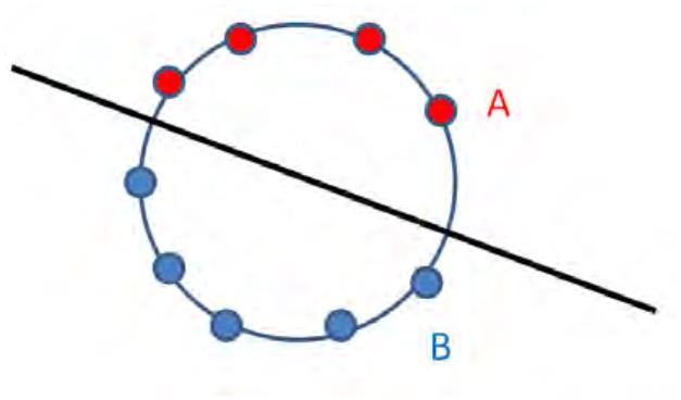


Randomized Hyperplane Rounding
given: one vector x for each i ∈ V
i
choose a random unit vector r ∈ Rn
set A = {i ∈ V : hx , ri ≥ 0}
i
set B = {i ∈ V : hx , ri < 0}
i
return the cut (A, B)
Thus, vertices are partitioned according to which side of the hyperplane with normal vector
r they lie on. You may be wondering how to choose a random unit vector in Rn in an
algorithm. One simple way is: sample n independent standard Gaussian random variables
(with mean 0 and variance 1) g , . . . , g , and normalize to get a unit vector:
1
n
(g , . . . , g )
n
1
r =
.
k(g , . . . , g )k
1
n
(Or, note that the computed cut doesn’t change if we don’t bother to normalize.) The main
property we need of the distribution of r is spherical symmetry — that all vectors at a given
distance from the origin are equally likely.
We have the following remarkable theorem.
Theorem 3.1 The expected weight of the cut produced by randomized hyperplane rounding
is at least .878 times the maximum possible.
The theorem follows easily from the following lemma.
Lemma 3.2 For every edge (i, j) ∈ E of the input graph,
ꢀ
ꢁ
1
Pr[(i, j) is cut] ≥ .878 · (1 − hx , x i) .
i
j
2
|
{z
}
contribution to SDP
Proof of Theorem 3.1: We can derive
E[weight of (A, B)] =
X
wij · Pr[(i, j) is cut]
(i,j)∈E
.878 ·
ꢀ
ꢁ
X
1
2
≥
≥
(1 − hx , x i)
i
j
(i,j)∈E
.878 · OP T,
where the equation follows from linearity of expectation (using one indicator random variable
per edge), the first inequality from Lemma 3.2, and the second inequality from the fact that
the xi’s are an optimal solution to vector programming relaxation of the maximum cut
problem. ꢀ
7


We conclude by proving the key lemma.
Figure 3: x and x are placed on different sides of the cut with probability θ/π.
i
j
Proof of Lemma 3.2: Fix an edge (i, j) ∈ E. Consider the two-dimensional subspace (through
the origin) spanned by the vectors x and x . Since r was chosen from a spherically symmetric
i
distribution, its projection onto this subspace is also spherically symmetric — it’s equally
j
likely to point in any direction. The vertices x and x are placed on different sides of the
i
cut if and only if they are “split” by the projection of r. (Figure 3.) If we let θ denote the
j
angle between x and x in this subspace, then 2θ out of the 2π radians of possible directions
i
result in the edge (i, j) getting cut. So we know the cutting probability, as a function of θ:
j
θ
Pr[(i, j) is cut] =
.
π
1
2
− h
x , x ) as a function of θ. But remember from pre-
i
We still need to understand (1
i
j
calculus that hx , x i = kx kkx k cos θ. And since x and x are both unit vectors (in the
i
original space and also the subspace that they span), we have
j
i
j
i
j
1
(1 − hx , x i) = (1 cos θ).
1
2
−
i
j
2
The lemma thus boils down to verifying that
ꢂ
ꢃ
θ
≥
.878 · 1(1 − cos θ)
π
2
for all possible values of θ ∈ [0, π]. This inequality is easily seen by plotting both sides, or if
you’re a stickler for rigor, by computations familiar from first-year calculus. ꢀ
8
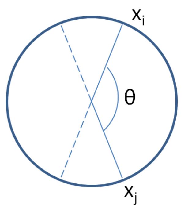


4
Going Beyond .878
For several lectures we were haunted by the number 1 − , which seemed like a pretty weird
1
e
number. Even more bizarrely, it is provably the best-possible approximation guarantee for
several natural problems, including online bipartite matching (Lecture #14) and, assuming
P = NP, set coverage (Lecture #15).
Now the .878 in this lecture seems like a really weird number. But there is some evidence
that it might be optimal! Specifically, in 2005 it was proved that, assuming that the “Unique
Games Conjecture (UGC)” is true (and P = NP), there is no polynomial-time algorithm
for the maximum cut problem with approximation factor larger than the one proved by
Goemans and Williamson. The UGC (which is only from 2002) is somewhat technical
to state precisely — it asserts that a certain constraint satisfaction problem is NP-hard.
Unlike the P = NP conjecture, which is widely believed, it is highly unclear whether the
UGC is true or false. But it’s amazing that any plausible complexity hypothesis implies the
optimality of randomized hyperplane rounding for the maximum cut problem.
9

CS261: A Second Course in Algorithms
The Top 10 List∗
Tim Roughgarden†
March 10, 2016
If you’ve kept up with this class, then you’ve learned a tremendous amount of material.
You know now more about algorithms than most people who don’t have a PhD in the field,
and are well prepared to tackle more advanced courses in theoretical computer science. To
recall how far you’ve traveled, let’s wrap up with a course top 10 list.
1
. The max-flow/min-cut theorem, and the corresponding polynomial-time algorithms for
computing them (augmenting paths, push-relabel, etc.). This is the theorem that se-
duced your instructor into a career in algorithms. Who knew that objects as seemingly
complex and practically useful as flows and cuts could be so beautifully characterized?
This theorem also introduced the running question of “how do we know when we’re
done?” We proved that a maximum flow algorithm is done (i.e., can correctly terminate
with the current flow) when the residual graph contains no s-t path or, equivalently,
when the current flow saturates some s-t cut.
2
3
. Bipartite matching, including the Hungarian algorithm for the minimum-cost perfect
bipartite matching problem. In this algorithm, we convinced ourselves we were done
by exhibiting a suitable dual solution (which at the time we called “vertex prices”)
certifying optimality.
. Linear programming is in P. We didn’t have time to go into the details of any lin-
ear programming algorithms, but just knowing this fact as a “black box” is already
extremely powerful. On the theoretical side, there are polynomial-time algorithms
for solving linear programs — even those whose constraints are specified implicitly
through a polynomial-time separation oracle — and countless theorems rely on this
fact. In practice, commercial linear program solvers routinely solve problem instances
with millions of variables and constraints and are a crucial tool in many real-world
applications.
∗
†
ꢀc
2
Department of Computer Science, Stanford University, 474 Gates Building, 353 Serra Mall, Stanford,
016, Tim Roughgarden.
CA 94305. Email: tim@cs.stanford.edu.
1

4
5
. Linear programming duality. For linear programming problems, there’s a generic way
to know when you’re done. Whatever the optimal solution of the linear program is,
strong LP duality guarantees that there’s a dual solution that proves its optimality.
While powerful and perhaps surprising, the proof of strong duality boils down to the
highly intuitive statement that, given a closed convex set and a point not in the set,
there’s a hyperplane with the set on one side and the point on the other.
. Online algorithms. It’s easy to think of real-world situations where decisions need to be
made before all of the relevant information is available. In online algorithms, the input
arrives “online” in pieces, and an irrevocable decision must be made at each time step.
For some problems, there are online algorithms with good (close to 1) competitive
ratios — algorithms that compute a solution with objective function value close to
that of the optimal solution. Such algorithms perform almost as well as if the entire
input was known in advance. For example, in online bipartite matching, we achieved
a competitive ratio of 1 −
1
e
≈
63% (which is the best possible).
6
. The multiplicative weights algorithm. This simple online algorithm, in the spirit of “re-
inforcement learning,” achieves per-time-step regret approaching 0 as the time horizon
T approaches infinity. That is, the algorithm does almost as well as the best fixed
action in hindsight. This result is interesting in its own right as a strategy for making
decisions over time. It also has some surprising applications, such as a proof of the
minimax theorem for zero-sum games (if both players randomize optimally, then it
doesn’t matter who goes first) and fast approximation algorithms for several problems
(maximum flow, multicommodity flow, etc.).
7
. The Traveling Salesman Problem (TSP). The TSP is a famous NP-hard problem with
a long history, and several of the most notorious open problems in approximation
algorithms concern different variants of the TSP. For the metric TSP, you now know
3
the state-of-the-art — Christofides’s -approximation algorithm, which is nearly 40
years old. Most researchers believe that better approximation algorithms exist. (You
2
also know close to the state-of-the-art for asymmetric TSP, where again it seems that
better approximation algorithms should exist.)
8
. Linear programming and approximation algorithms. Linear programs are useful not
only for solving problems exactly in polynomial time, but also in the design and analysis
of polynomial-time approximation algorithms for NP-hard optimization problems. In
some cases, linear programming is used only in the analysis of an algorithm, and
not explicitly in the algorithm itself. A good example is our analysis of the greedy
set cover algorithm, where we used a feasible dual solution as a lower bound on the
cost of an optimal set cover. In other applications, such as vertex cover and low-
congestion routing, the approximation algorithm first explicitly solves an LP relaxation
of the problem, and then “rounds” the resulting fractional solution into a near-optimal
integral solution. Finally, some algorithms, like our primal-dual algorithm for vertex
2

cover, use linear programs to guide their decisions, without ever explicitly or exactly
solving the linear programs.
9
. Five essential tools for the analysis of randomized algorithms. And in particular, the
Chernoff bounds, which prove sharp concentration around the expected value for ran-
dom variables that are sums of bounded independent random variables. Chernoff
bounds are used all the time. We saw an application in randomized rounding, leading
to a O(log n/ log log n)-approximation algorithm for low-congestion routing.
We also reviewed four easy-to-prove tools that you’ve probably seen before: linearity of
expectation (which is trivial but super-useful), Markov’s inequality (which is good for
constant-probability bounds), Chebyshev’s inequality (good for random variables with
small variance), and the union bound (which is good for avoiding lots of low-probability
events simultaneously).
1
0. Beating brute-force search. NP-hardness is not a death sentence — it just means that
you need to make some compromises. In approximation algorithms, one insists on a
polynomial running time and compromises on correctness (i.e., on exact optimality).
But one can also insist on correctness, resigning oneself to an exponential running time
(but still as fast as possible). We saw three examples of NP-hard problems that admit
exact algorithms that are significantly faster than brute-force search: the unweighted
vertex cover problem (an example of a “fixed-parameter tractable” algorithm, with
running time of the form poly(n) + f(k) rather than O(nk)); TSP (where dynamic
programming reduces the running time from roughly O(n!) to roughly O(2n)); and
3
SAT (where random search reduces the running time from roughly O(2n) to roughly
O((4/3)n)).
3
CS261: Exercise Set #1
For the week of January 4–8, 2016
Instructions:
(1) Do not turn anything in.
(2) The course staff is happy to discuss the solutions of these exercises with you in office hours or on
Piazza.
(3) While these exercises are certainly not trivial, you should be able to complete them on your own
(perhaps after consulting with the course staff or a friend for hints).
Exercise 1
Suppose we generalize the maximum flow problem so that there are multiple source vertices s , . . . , s ∈ V
1
k
and sink vertices t , . . . , t ∈ V . (As usual, the rest of the input is a directed graph with integer edge
1
`
capacities.) You should assume that no vertex is both a source and sink, that source vertices have no
incoming edges, and that sink vertices have no outgoing edges. A flow is defined as before: a nonnegative
number f for each e ∈ E such that capacity constraints are obeyed on every edge and such that conservation
e
constraints hold at all vertices that are neither a source nor a sink. The value of a flow is the total amount
P
P
of outgoing flow at the sources:
k
i=1
f .
e∈δ (s )
+
e
i
Prove that the maximum flow problem in graphs with multiple sources and sinks reduces to the single-
source single-sink version of the problem. That is, given an instance of the multi-source multi-sink version
of the problem, show how to (i) produce a single-source single-sink instance such that (ii) given a maximum
flow to this single-source single-sink instance, you can recover a maximum flow of the original multi-source
multi-sink instance. Your implementations of steps (i) and (ii) should run in linear time. Include a brief
proof of correctness.
[
Hint: consider adding additional vertices and/or edges.]
Exercise 2
In lecture we’ve focused on the maximum flow problem in directed graphs. In the undirected version of the
problem, the input is an undirected graph G = (V, E), a source vertex s ∈ V , a sink vertex t ∈ V , and a
integer capacity u ≥ 0 for each edge e ∈ E.
e
Flows are defined exactly as before, and remain directed. Formally, a flow consists of two nonnegative
numbers fuv and fvu for each (undirected) edge (u, v) ∈ E, indicating the amount of traffic traversing
the edge in each direction. Conservation constraints (flow in = flow out) are defined as before. Capacity
constraints now state that, for every edge e = (u, v) ∈ E, the total amount of flow f + fvu on the edge is
P
uPv
at most the edge’s capacity u . The value of a flow is the net amount
of the source.
Prove that the maximum flow problem in undirected graphs reduces to the maximum flow problem in
directed graphs. That is, given an instance of the undirected problem, show how to (i) produce an instance
of the directed problem such that (ii) given a maximum flow to this directed instance, you can recover a
maximum flow of the original undirected instance. Your implementations of steps (i) and (ii) should run in
linear time. Include a brief proof of correctness.
f
−
fvs going out
e
(s,v)∈E sv
(v,s)∈E
[
Hint: consider bidirecting each edge.]
1
Exercise 3
For every positive integer U, show that there is an instance of the maximum flow problem with edge capacities
in {1, 2, . . . , U} and a choice of augmenting paths so that the Ford-Fulkerson algorithm runs for at least U
iterations before terminating. The number of vertices and edges in your networks should be bounded above
by constant, independent of U. (This shows that the algorithm is only “pseudopolynomial.”)
[
Hint: use a network similar to the examples discussed in lecture.]
Exercise 4
Consider the special case of the maximum flow problem in which every edge has capacity 1. (This is called
the unit-capacity case.) Explain why a suitable implementation of the Ford-Fulkerson algorithm runs in
O(mn) time in this special case. (As always, m denotes the number of edges and n the number of vertices.)
Exercise 5
Consider a directed graph G = (V, E) with source s and sink t for which each edge e has a positive integral
capacity u . For a flow f in G, define the “layered graph” L as in Lecture #2, by computing the residual
e
f
graph G and running breadth-first search (BFS) in G starting from s, aborting once the sink t is reached,
f
f
and retaining only the forward edges. (Recall that a forward edge in BFS goes from layer i to layer (i + 1),
for some i.)
Recall from Lecture #2 that a blocking flow in a network is a flow that saturates at least one edge on each
s-t path. Prove that for every flow f and every blocking flow g in Lf , the shortest-path distance between s
and t in the new residual graph Gf+g is strictly larger than that in Gf .
2
CS261: Exercise Set #2
For the week of January 11–15, 2016
Instructions:
(1) Do not turn anything in.
(2) The course staff is happy to discuss the solutions of these exercises with you in office hours or on
Piazza.
(3) While these exercises are certainly not trivial, you should be able to complete them on your own
(perhaps after consulting with the course staff or a friend for hints).
Exercise 6
In the s-t directed edge-disjoint paths problem, the input is a directed graph G = (V, E), a source vertex s,
and a sink vertex t. The goal is to output a maximum-cardinality set of edge-disjoint s-t paths P , . . . , P .
1
k
(I.e., P and P should share no edges for each i = j, and k should be as large as possible.)
i
j
Prove that this problem reduces to the maximum flow problem. That is, given an instance of the disjoint
paths problem, show how to (i) produce an instance of the maximum flow problem such that (ii) given a
maximum flow to this instance, you can compute an optimal solution to the disjoint paths instance. Your
implementations of steps (i) and (ii) should run in linear and polynomial time, respectively. (Can you achieve
linear time also for (ii)?) Include a brief proof of correctness.
[
Hint: for (ii), make use of your solution to Problem 1 (from Problem Set #1).]
Exercise 7
In the s-t directed vertex-disjoint paths problem, the input is a directed graph G = (V, E), a source vertex s,
and a sink vertex t. The goal is to output a maximum-cardinality set of internally vertex-disjoint s-t paths
P , . . . , P . (I.e., P and P should share no vertices other than s and t for each i = j, and k should be as
1
k
i
j
large as possible.) Give a polynomial-time algorithm for this problem.
[
Hint: reduce the problem either directly to the maximum flow problem or to the edge-disjoint version solved
in the previous exercise.]
Exercise 8
In the (undirected) global minimum cut problem, the input is an undirected graph G = (V, E) with a
nonnegative capacity u for each edge e ∈ E, and the goal is to identify a cut (A, B) — i.e., a partition of V
e
P
into non-empty sets A and B — that minimizes the total capacity
u of the cut edges. (Here, δ(A)
e
e∈δ(S)
denotes the edges with exactly one endpoint in A.)
Prove that this problem reduces to solving n−1 maximum flow problems in undirected graphs.1 That is,
given an instance the global minimum cut problem, show how to (i) produce n−1 instances of the maximum
flow problem (in undirected graphs) such that (ii) given maximum flows to these n − 1 instances, you can
compute an optimal solution to the global minimum cut instance. Your implementations of steps (i) and (ii)
should run in polynomial time. Include a brief proof of correctness.
1
And hence to solving n − 1 maximum flow problems in directed graphs.
1

Exercise 9
Extend the proof of Hall’s Theorem (end of Lecture #4) to show that, for every bipartite graph G =
(V ∪ W, E) with |V | ≤ |W|,
maximum cardinality of a matching in G = Sm⊆iVn [|V | − (|S| − |N(S)|)] .
Exercise 10
In lecture we proved a bound of O(n3) on the number of operations needed by the Push-Relabel algorithm
(where each iteration, we select the highest vertex with excess to Push or Relabel) before it terminates with
a maximum flow. Give an implementation of this algorithm that runs in O(n3) time.
[
Hints: first prove the running time bound assuming that, in each iteration, you can identify the highest
vertex with positive excess in O(1) time. The hard part is to maintain the vertices with positive excess in a
data structure such that, summed over all of the iterations of the algorithm, only O(n3) total time is used
to identify these vertices. Can you get away with just a collection of buckets (implemented as lists), sorted
by height?]
2
CS261: Exercise Set #3
For the week of January 18–22, 2016
Instructions:
(1) Do not turn anything in.
(2) The course staff is happy to discuss the solutions of these exercises with you in office hours or on
Piazza.
(3) While these exercises are certainly not trivial, you should be able to complete them on your own
(perhaps after consulting with the course staff or a friend for hints).
Exercise 11
Recall that in the maximum-weight bipartite matching problem, the input is a bipartite graph G = (V ∪W, E)
P
with a nonnegative weight w per edge, and the goal is to compute a matching M that maximizes
w .
e
e∈M
e
In the minimum-cost perfect bipartite matching problem, the input is a bipartite graph G = (V ∪ W, E)
such that |V | = |W| and G contains a perfect matching, and a nonnegative cost c per edge, and the goal is
P
e
to compute a perfect matching M that minimizes
c .
e∈M
e
Give a linear-time reduction from the former problem to the latter problem.
Exercise 12
Suppose you are given an undirected bipartite graph G = (V ∪ W, E) and a positive integer bv for every
vertex v ∈ V ∪ W. A b-matching is a subset M ⊆ E of edges such that each vertex v is incident to at most
b edges of M. (The standard bipartite matching problem corresponds to the case where b = 1 for every
v
v
v ∈ V ∪ W.)
Prove that the problem of computing a maximum-cardinality bipartite b-matching reduces to the problem
of computing a (standard) maximum-cardinality bipartite matching in a bigger graph. Your reduction should
run in time polynomial in the size of G and in maxv∈V ∪W bv.
Exercise 13
A graph is d-regular if every vertex has d incident edges. Prove that every d-regular bipartite graph is the
union of d perfect matchings. Does the same statement hold for d-regular non-bipartite graphs?
[
Hint: Hall’s theorem.]
Exercise 14
Prove that the minimum-cost perfect bipartite matching problem reduces, in linear time, to the minimum-
cost flow problem defined in Lecture #6.
1
Exercise 15
In the edge cover problem, the input is a graph G = (V, E) (not necessarily bipartite) with no isolated
vertices, and the goal is to compute a minimum-cardinality subset F ⊆ E of edges such every vertex v ∈ V
is the endpoint of at least one edge in F. Prove that this problem reduces to the maximum-cardinality
(non-bipartite) matching problem.
2
CS261: Exercise Set #4
For the week of January 25–29, 2016
Instructions:
(1) Do not turn anything in.
(2) The course staff is happy to discuss the solutions of these exercises with you in office hours or on
Piazza.
(3) While these exercises are certainly not trivial, you should be able to complete them on your own
(perhaps after consulting with the course staff or a friend for hints).
Exercise 16
In Lecture #7 we noted that the maximum flow problem translates quite directly into a linear program:
X
max
fe
e∈δ (s)
+
subject to
X
X
fe −
fe = 0
f ≤ u
for all v = s, t
e∈δ−(v)
e∈δ (v)
+
for all e ∈ E
for all e ∈ E.
e
e
f ≥ 0
e
(As usual, we are assuming that s has no incoming edges.) In Lecture #8 we considered the following
alternative linear program, where P denotes the set of s-t paths of G:
X
max
fP
P ∈P
subject to
X
fP ≤ ue
fP ≥ 0
for all e ∈ E
for all P ∈ P.
P ∈P : e∈P
Prove that these two linear programs always have equal optimal objective function value.
Exercise 17
In the multicommodity flow problem, the input is a directed graph G = (V, E) with k source vertices s , . . . , s ,
1
k
k sink vertices t , . . . , t , and a nonnegative capacity u for each edge e ∈ E. An s -t pair is called a
1
k
e
i
i
commodity. A multicommodity flow if a set of k flows f(1), . . . , f(k) such that (i) for each i = 1, 2, . . . , k, f(i)
is an s -t flow (in the usual max flow sense); and (ii) for every edge e, the total amount of flow (summing
i
i
over all commodities) sent on e is at most the edge capacity u . The value of a multicommodity flow is the
e
sum of the values (in the usual max flow sense) of the flows f(1), . . . , f(k).
Prove that the problem of finding a multicommodity flow of maximum-possible value reduces in polyno-
mial time to solving a linear program.
1
Exercise 18
Consider a primal linear program (P) of the form
max cT x
subject to
Ax = b
x ≥ 0.
The recipe from Lecture #8 gives the following dual linear program (D):
min bT y
subject to
AT y ≥ c
y ∈ R.
Prove weak duality for primal-dual pairs of this form: the (primal) objective function value of every
feasible solution to (P) is bounded above by the (dual) objective function value of every feasible solution
to (D).1
Exercise 19
Consider a primal linear program (P) of the form
max cT x
subject to
Ax ≤ b
x ≥ 0
and corresponding dual program (D)
min bT y
subject to
AT y ≥ c
y ≥ 0.
Suppose xˆ and yˆ are feasible for (P) and (D), respectively. Prove that if xˆ, yˆ do not satisfy the complementary
slackness conditions, then cT xˆ = bT yˆ.
Exercise 20
Recall the linear programming relaxation of the minimum-cost bipartite matching problem:
X
min
c x
e e
e∈E
1
In Lecture #8, we only proved weak duality for primal linear programs with only inequality constraints (and hence dual
programs with nonnegative variables), like those in Exercise 19.
2

subject to
X
xe = 1
xe ≥ 0
for all v ∈ V ∪ W
for all e ∈ E.
e∈δ(v)
In Lecture #8 we appealed to the Hungarian algorithm to prove that this linear program is guaranteed to
have an optimal solution that is 0-1. This point of this exercise is to give a direct proof of this fact, without
recourse to the Hungarian algorithm.
(a) By a fractional solution, we mean a feasible solution to the above linear program such that 0 < xe < 1
for some edge e ∈ E. Prove that, for every fractional solution, there is an even cycle C of edges with
0
< x < 1 for every e ∈ C.
e
(b) Prove that, for all ꢀ sufficiently close to 0 (positive or negative), adding ꢀ to xe for every other edge
of C and subtracting ꢀ from xe for the other edges of C yields another feasible solution to the linear
program.
(c) Show how to transform a fractional solution x into another fractional solution x0 such that: (i) x0 has
fewer fractional coordinates than x; and (ii) the objective function value of x0 is no larger than that
of x.
(d) Conclude that the linear programming relaxation above is guaranteed to possess an optimal solution
that is 0-1 (i.e., not fractional).
3
CS261: Exercise Set #5
For the week of February 1–5, 2016
Instructions:
(1) Do not turn anything in.
(2) The course staff is happy to discuss the solutions of these exercises with you in office hours or on
Piazza.
(3) While these exercises are certainly not trivial, you should be able to complete them on your own
(perhaps after consulting with the course staff or a friend for hints).
Exercise 21
Consider the following linear programming relaxation of the maximum-cardinality matching problem:
X
max
xe
e∈E
subject to
X
xe ≤ 1
for all v ∈ V
for all e ∈ E,
e∈δ(v)
xe ≥ 0
where δ(v) denotes the set of edges incident to vertex v.
We know from Lecture #9 that for bipartite graphs, this linear program always has an optimal 0-1
solution. Is this also true for non-bipartite graphs?
Exercise 22
Let x1, . . . , xn ∈ Rm be a set of n m-vectors. Define C as the cone of x , . . . , x , meaning all linear
1
n
combinations of the x ’s that use only nonnegative coefficients:
i
(
)
Xn
C =
λ x : λ , . . . , λ ≥ 0
.
i
i
1
n
i=1
Suppose α ∈ Rm, β ∈ R define a “valid inequality” for C, meaning that
αT x ≥ β
for every x ∈ C. Prove that
αT x
≥
0
for every x ∈ C, so α and 0 also define a valid inequality.
[
Hint: Show that β > 0 is impossible. Then use the fact that if x ∈ C then λx ∈ C for all scalars λ ≥ 0.]
1
Exercise 23
Verify that the two linear programs discussed in the proof of the minimax theorem (Lecture #10),
max v
subject to
Xm
v −
a x ≤ 0
for all j = 1, . . . , n
for all i = 1, . . . , m
ij
i
i=1
Xm
xi = 1
x ≥ 0
i=1
i
v ∈ R,
and
min w
subject to
Xn
w −
a y ≥ 0
for all i = 1, . . . , m
for all j = 1, . . . , n
ij
j
j=1
Xn
yj = 1
y ≥ 0
j=1
j
w ∈ R,
are both feasible and are dual linear programs. (As in lecture, A is an m × n matrix, with a specifying the
ij
payoff of the row player and the negative of the payoff of the column player when the former chooses row i
and the latter chooses column j.)
Exercise 24
Consider a linear program with n decision variables, and a feasible solution x ∈ Rn at which less than n of
the constraints hold with equality (i.e., the rest of the constraints hold as strict inequalities).
(a) Prove that there is a direction y ∈ Rn such that, for all sufficiently small ꢀ > 0, x + ꢀy and x − ꢀy are
both feasible.
(b) Prove that at least one of x + ꢀy, x − ꢀy has objective function value at least as good as x.
[
Context: these are the two observations that drive the fact that a linear program with a bounded feasible
region always has an optimal solution at a vertex. Do you see why?]
Exercise 25
Recall from Problem #12(e) (in Problem Set #2) the following linear programming formulation of the s-t
shortest path problem:
X
min
c x
e e
e∈E
2
subject to
X
xe ≥ 1
xe ≥ 0
for all S ⊆ V with s ∈ S, t ∈/ S
for all e ∈ E.
e∈δ (S)
+
Prove that this linear program, while having exponentially many constraints, admits a polynomial-time
separation oracle (in the sense of the ellipsoid method, see Lecture #10).
3
CS261: Exercise Set #6
For the week of February 8–12, 2016
Instructions:
(1) Do not turn anything in.
(2) The course staff is happy to discuss the solutions of these exercises with you in office hours or on
Piazza.
(3) While these exercises are certainly not trivial, you should be able to complete them on your own
(perhaps after consulting with the course staff or a friend for hints).
Exercise 26
In the online-decision making problem (Lecture #11), suppose that you know in advance an upper bound
P
Q on the sum of squared rewards (
multiplicative weights algorithm and analysis to obtain a regret bound of O( Q log n + log n).
T
t=1
r a
( t( ))2) for every action
a ∈ A
. Explain how to modify the
√
Exercise 27
Consider the thought experiment sketched at the end of Lecture #11: for a zero-sum game specified by the
n × n matrix A:
•
At each time step t = 1, 2, . . . , T = 4 ln n :
2
ꢀ
–
–
–
The row and column players each choose a mixed strategy (pt and qt, respectively) using their own
copies of the multiplicative weights algorithm (with the action set equal to the rows or columns,
as appropriate).
The row player feeds the reward vector rt = Aqt into (its copy of) the multiplicative weights
algorithm. (This is just the expected payoff of each row, given that the column player chose the
mixed strategy qt.)
The column player feeds the reward vector rt = −(pt)T A into the multiplicative weights algo-
rithm.
Let
1
XT
v =
(pt)T Aqt
T
t=1
denote the time-averaged payoff of the row player. Use the multiplicative weights guarantee for the row and
column players to prove that
ꢀ
ꢁ
v ≥ max p
T A qˆ
− ꢀ
p
and
ꢀ
ꢁ
v ≤ min pˆ
T Aq
+
ꢀ,
q
P
P
respectively, where pˆ = T1
T
t=1
pt and qˆ = T1
T
t=1
qt denote the time-averaged row and column strategies.
[
Hint: first consider the maximum and minimum over all deterministic row and column strategies, respec-
tively, rather than over all mixed strategies p and q.]
1


Exercise 28
Use the previous exercise to prove the minimax theorem:
ꢀ
ꢁ
ꢀ
ꢁ
max min pT Aq = min max pT Aq
p
q
q
p
for every zero-sum game A.
Exercise 29
There are also other notions of regret. One useful one is swap regret, which for an action sequence a1, . . . , aT
and a reward vector sequence r1, . . . , rT is defined as
XT
XT
max
δ:A→A
rt(δ(at)) −
rt(at)
t=1
t=1
where the maximum ranges over all functions from A to itself. Thus the swap regret measures how much
better you could do in hindsight by, for each action a, switching your action from a to some other action (on
the days where you previously chose a). Prove that, even with just 3 actions, the swap regret of an action
sequence can be arbitrarily larger (as T → ∞) than the standard regret (as defined in Lecture #11).1
Exercise 30
At the end of Lecture #12 we showed how to use the multiplicative weights algorithm (as a black box) to
2
obtain a (1 − ꢀ)-approximate maximum flow in O(OP T log n) iterations in networks where all edges have
2
ꢀ
capacity 1. (We are ignoring the outer loop that does binary search on the value of OPT.) Extend this idea
to obtain the same result for maximum flow instances in which every edge capacity is at least 1.
P
[
Hint: if {`∗}
is an optimal dual solution, with value OPT =
c `∗, then obtain a distribution by
e
e∈E
e∈E
e
e
scaling each c `∗ down by OPT. What are the relevant edge lengths after this scaling?]
e
e
1
Despite this, there are algorithms (a bit more complicated than multiplicative weights, but still reasonably simple) that
guarantee swap regret sublinear in T.
2


CS261: Exercise Set #7
For the week of February 15–19, 2016
Instructions:
(1) Do not turn anything in.
(2) The course staff is happy to discuss the solutions of these exercises with you in office hours or on
Piazza.
(3) While these exercises are certainly not trivial, you should be able to complete them on your own
(perhaps after consulting with the course staff or a friend for hints).
Exercise 31
Recall Graham’s algorithm from Lecture #13: given a parameter m (the number of machines) and n jobs
arriving online with processing times p , . . . , p , always assign the current job to the machine that currently
1
n
has the smallest load. We proved that the schedule produced by this algorithm always has makespan (i.e.,
maximum machine load) at most twice the minimum possible in hindsight.
Show that for every constant c < 2, there exists an instance for which the schedule produced by Graham’s
algorithm has makespan more than c times the minimum possible.
[
Hint: Your bad instances will need to grow larger as c approaches 2.]
Exercise 32
In Lecture #13 we considered the online Steiner tree problem, where the input is a connected undirected
graph G = (V, E) with nonnegative edge costs c , and a sequence t , . . . , t ∈ V of “terminals” arrive
e
1
k
online. The goal is to output a subgraph that spans all the terminals and has total cost as small as possible.
In lecture we only considered the metric special case, where the graph G is complete and the edge costs
satisfy the triangle inequality. (I.e., for every triple u, v, w ∈ V , c
≤ c + cvw.) Show how to convert
uw
uv
an α-competitive online algorithm for the metric Steiner tree problem into one for the general Steiner tree
problem.1
[
Hint: Define a metric instance where the edges represent paths in the original (non-metric) instance.]
Exercise 33
Give an infinite family of instances (with the number k of terminals tending to infinity) demonstrating that
the greedy algorithm for the online Steiner tree problem is Ω(log k)-competitive (in the worst case).
Exercise 34
Let G = (V, E) be an undirected graph that is connected and Eulerian (i.e., all vertices have even degree).
Show that G admits an Euler tour — a (not necessarily simple) cycle that uses every edge exactly once. Can
you turn your proof into an O(m)-time algorithm, where m = |E|?
[
Hint: Induction on |E|.]
1
This extends the 2 ln k competitive ratio given in lecture to the general online Steiner tree problem.
1

Exercise 35
Consider the following online matching problem in general, not necessarily bipartite graphs. No information
about the graph G = (V, E) is given up front. Vertices arrive one-by-one. When a vertex v ∈ V arrives, and
S ⊆ V are the vertices that arrived previously, the algorithm learns about all of the edges between v and
vertices in S. Equivalently, after i time steps, the algorithm knows the graph G[S ] induced by the set S of
i
i
the first i vertices.
Give a 12 -competitive online algorithm for this problem.
2

CS261: Exercise Set #8
For the week of February 22–26, 2016
Instructions:
(1) Do not turn anything in.
(2) The course staff is happy to discuss the solutions of these exercises with you in office hours or on
Piazza.
(3) While these exercises are certainly not trivial, you should be able to complete them on your own
(perhaps after consulting with the course staff or a friend for hints).
Exercise 36
Recall the MST heuristic for the Steiner tree problem — in Lecture #15, we showed that this is a 2-
approximation algorithm. Show that, for every constant c < 2, there is an instance of the Steiner tree
problem such that the MST heuristic returns a tree with cost more than c times that of an optimal Steiner
tree.
Exercise 37
Recall the greedy algorithm for set coverage (Lecture #15). Prove that for every k ≥ 1, there is an example
where the value of the greedy solution is at most 1 − (1 − 1 )k times that of an optimal solution.
k
Exercise 38
Recall the MST heuristic for the metric TSP problem — in Lecture #16, we showed that this is a 2-
approximation algorithm. Show that, for every constant c < 2, there is an instance of the metric TSP
problem such that the MST heuristic returns a tour with cost more than c times the minimum possible.
Exercise 39
Recall Christofides’s 3 -approximation algorithm for the metric TSP problem. Prove that the analysis given
2
in Lecture #16 is tight: for every constant c < 3 , there is an instance of the metric TSP problem such that
2
Christofides’s algorithm returns a tour with cost more than c times the minimum possible.
Exercise 40
Consider the following variant of the traveling salesman problem (TSP). The input is an undirected complete
graph with edge costs. These edge costs need not satisfy the triangle inequality. The desired output is the
minimum-cost cycle, not necessarily simple, that visits every vertex at least once.
Show how to convert a polynomial-time α-approximation algorithm for the metric TSP problem into a
polynomial-time α-approximation algorithm for this (non-metric) TSP problem with repeated visits allowed.
[
Hint: Compare to Exercise 32.]
1


CS261: Exercise Set #9
For the week of February 29–March 4, 2016
Instructions:
(1) Do not turn anything in.
(2) The course staff is happy to discuss the solutions of these exercises with you in office hours or on
Piazza.
(3) While these exercises are certainly not trivial, you should be able to complete them on your own
(perhaps after consulting with the course staff or a friend for hints).
Exercise 41
Recall the Vertex Cover problem from Lecture #17: the input is an undirected graph G = (V, E) and a
non-negative cost cv for each vertex v ∈ V . The goal is to compute a minimum-cost subset S ⊆ V that
includes at least one endpoint of each edge.
The natural greedy algorithm is:
•
•
S = ∅
while S is not a vertex cover:
–
add to S the vertex v minimizing (cv/# newly covered edges)
•
return S
Prove that this algorithm is not a constant-factor approximation algorithm for the vertex cover problem.
Exercise 42
Recall from Lecture #17 our linear programming relaxation of the Vertex Cover problem (with nonnegative
edge costs):
X
min
c x
v v
v∈V
subject to
and
xv + xw ≥ 1
xv ≥ 0
for all edges e = (v, w) ∈ E
for all vertices v ∈ V .
Prove that there is always a half-integral optimal solution x∗ of this linear program, meaning that x∗ ∈
v
{
0, 1 , 1} for every v ∈ V .
2
[
Hint: start from an arbitrary feasible solution and show how to make it “closer to half-integral” while only
improving the objective function value.]
1

Exercise 43
Recall the primal-dual algorithm for the vertex cover problem — in Lecture #17, we showed that this is a
2
-approximation algorithm. Show that, for every constant c < 2, there is an instance of the vertex cover
problem such that this algorithm returns a vertex cover with cost more than c times that of an optimal
vertex cover.
Exercise 44
Prove Markov’s inequality: if X is a non-negative random variable with finite expectation and c > 1, then
1
Pr[X ≥ c · E[X]] ≤
.
c
Exercise 45
ꢀ
ꢁ
Let X be a random variable with finite expectation and variance; recall that Var[X] = E (X − E[X])2 and
p
StdDev[X] = Var[X]. Prove Chebyshev’s inequality: for every t > 1,
1
Pr[|X − E[X] | ≥ t · StdDev[X]] ≤
.
t2
[
Hint: apply Markov’s inequality to the (non-negative!) random variable (X − E[X])2.]
2


CS261: Problem Set #1
Due by 11:59 PM on Tuesday, January 26, 2016
Instructions:
(1) Form a group of 1-3 students. You should turn in only one write-up for your entire group.
(2) Submission instructions: We are using Gradescope for the homework submissions. Go to www.gradescope.com
to either login or create a new account. Use the course code 9B3BEM to register for CS261. Only one
group member needs to submit the assignment. When submitting, please remember to add all group
member names in Gradescope.
(3) Please type your solutions if possible and we encourage you to use the LaTeX template provided on
the course home page.
(4) Write convincingly but not excessively.
(5) Some of these problems are difficult, so your group may not solve them all to completion. In this case,
you can write up what you’ve got (subject to (3), above): partial proofs, lemmas, high-level ideas,
counterexamples, and so on.
(6) Except where otherwise noted, you may refer to the course lecture notes only. You can also review any
relevant materials from your undergraduate algorithms course.
(7) You can discuss the problems verbally at a high level with other groups. And of course, you are
encouraged to contact the course staff (via Piazza or office hours) for additional help.
(8) If you discuss solution approaches with anyone outside of your group, you must list their names on the
front page of your write-up.
(9) Refer to the course Web page for the late day policy.
Problem 1
This problem explores “path decompositions” of a flow. The input is a flow network (as usual, a directed
graph G = (V, E), a source s, a sink t, and a positive integral capacity ue for each edge), as well as a flow f
in G. As always with graphs, m denotes |E| and n denotes |V |.
(a) A flow is acyclic if the subgraph of directed edges with positive flow contains no directed cycles. Prove
that for every flow f, there is an acyclic flow with the same value of f. (In particular, this implies that
some maximum flow is acyclic.)
(b) A path flow assigns positive values only to the edges of one simple directed path from s to t. Prove
that every acyclic flow can be written as the sum of at most m path flows.
(c) Is the Ford-Fulkerson algorithm guaranteed to produce an acyclic maximum flow?
(d) A cycle flow assigns positive values only to the edges of one simple directed cycle. Prove that every
flow can be written as the sum of at most m path and cycle flows.
(e) Can you compute the decomposition in (d) in O(mn) time?
1
Problem 2
Consider a directed graph G = (V, E) with source s and sink t for which each edge e has a positive integral
capacity u . Recall from Lecture #2 that a blocking flow in such a network is a flow {f }
e∈E
with the
property that, for every s-t path P of G, there is at least one edge of P such that f = u . For example, our
e
e
e
e
first (broken) greedy algorithm from Lecture #1 terminates with a blocking flow (which, as we saw, is not
necessarily a maximum flow).
Dinic’s Algorithm
initialize f = 0 for all e ∈ E
e
while there is an s-t path in the current residual network G do
f
construct the layered graph L , by computing the residual graph G and running
f
f
breadth-first search (BFS) in Gf starting from s, stopping once the sink t is
reached, and retaining only the forward edges1
compute a blocking flow g in Gf
/
/ augment the flow f using the flow g
for all edges (v, w) of G for which the corresponding forward edge of Gf carries
flow (gvw > 0) do
increase fe by ge
for all edges (v, w) of G for which the corresponding reverse edge of Gf carries
flow (gwv > 0) do
decrease fe by ge
The termination condition implies that the algorithm can only halt with a maximum flow. Exercise Set #1
argues that every iteration of the main loop increases d(f), the length (i.e., number of hops) of a shortest
s-t path in Gf , and therefore the algorithm stops after at most n iterations. Its running time is therefore
O(n·BF), where BF is the amount of time required to compute a blocking flow in the layered graph L . We
f
know that BF = O(m2) — our first broken greedy algorithm already proves this — but we can do better.
Consider the following algorithm, inspired by depth-first search, for computing a blocking flow in Lf :
A Blocking Flow Algorithm
Initialize. Initialize the flow variables g to 0 for all e ∈ E. Initialize the path variable
e
P as the empty path, from s to itself. Go to Advance.
Advance. Let v denote the current endpoint of the path P. If there is no edge out
of v, go to Retreat. Otherwise, append one such edge (v, w) to the path P. If w = t
then go to Advance. If w = t then go to Augment.
Retreat. Let v denote the current endpoint of the path P. If v = s then halt.
Otherwise, delete v and all of its incident edges from Lf . Remove from P its last edge.
Go to Advance.
Augment. Let ∆ denote the smallest residual capacity of an edge on the path P
(which must be an s-t path). Increase g by ∆ on all edges e ∈ P. Delete newly
e
saturated edges from L , and let e = (v, w) denote the first such edge on P. Retain
f
only the subpath of P from s to v. Go to Advance.
And now the analysis:
(a) Prove that the running time of the algorithm, suitably implemented, is O(mn). (As always, m denotes
|
E| and n denotes |V |.)
Hint: How many times can Retreat be called? How many times can Augment be called? How many
[
times can Advance be called before a call to Retreat or Augment?]
1
Recall that a forward edge in BFS goes from layer i to layer (i + 1), for some i.
2


(b) Prove that the algorithm terminates with a blocking flow g in Lf .
For example, you could argue by contradiction.]
[
(c) Suppose that every edge of Lf has capacity 1 (cf., Exercise #4). Prove that the algorithm above
computes a blocking flow in linear (i.e., O(m)) time.
[
Hint: can an edge (v, w) be chosen in two different calls to Advance?]
Problem 3
In this problem we’ll analyze a different augmenting path-based algorithm for the maximum flow problem.
Consider a flow network with integral edge capacities. Suppose we modify the Edmonds-Karp algorithm
(Lecture #2) so that, instead of choosing a shortest augmenting path in the residual network Gf , it chooses
an augmenting path on which it can push the most flow. (That is, it maximizes the minimum residual
capacity of an edge in the path.) For example, in the network in Figure 1, this algorithm would push 3 units
of flow on the path s → v → w → t in the first iteration. (And 2 units on s → w → v → t in the second
iteration.)
v
3
(3)
2
s
5 (3)
t
2
3 (3)
w
Figure 1: Problem 3. Edges are labeled with their capacities, with flow amounts in parentheses.
(a) Show how to modify Dijkstra’s shortest-path algorithm, without affecting its asymptotic running time,
so that it computes an s-t path with the maximum-possible minimum residual edge capacity.
(b) Suppose the current flow f has value F and the maximum flow value in G is F∗. Prove that there
∗
−
is an augmenting path in Gf such that every edge has residual capacity at least (F
m = |E|.
F)/m, where
[
Hint: if ∆ is the maximum amount of flow that can be pushed on any s-t path of Gf , consider the set
of vertices reachable from s along edges in Gf with residual capacity more than ∆. Relate the residual
∗
−
capacity of this (s, t)-cut to F
F.]
(c) Prove that this variant of the Edmonds-Karp algorithm terminates within O(m log F∗) iterations,
where F∗ is defined as in the previous problem.
[
Hint: you might find the inequality 1 − x ≤ e− for x [0, 1] useful.]
x
∈
(d) Assume that all edge capacities are integers in {1, 2, . . . , U}. Give an upper bound on the running time
of your algorithm as a function of n = |V |, m, and U. Is this bound polynomial in the input size?
Problem 4
In this problem we’ll revisit the special case of unit-capacity networks, where every edge has capacity 1 (see
also Exercise 4).
3
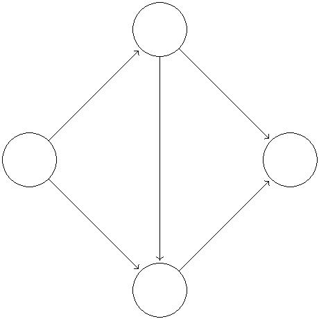
(a) Recall the notation d(f) for the length (in hops) of a shortest s-t path in the residual network Gf .
Suppose G is a unit-capacity network and f is a flow with value F. Prove that the maximum flow
m
d(f)
value is at most F +
.
[Hint: use the layered graph Lf discussed in Problem 2 to identify an s-t cut of the residual graph that
has small residual capacity. Then argue along the lines of Problem 3(b).]
(b) Explain how to compute a maximum flow in a unit-capacity network in O(m3/2) time.
[
Hints: use Dinic’s algorithm and Problem 2(c). Also, in light of part (a) of this problem, consider the
question: if you know that the value of the current flow f is only c less than the maximum flow value
in G, then what’s a crude upper bound on the number of additional blocking flows required before
you’re sure to terminate with a maximum flow?]
Problem 5
(Difficult.) This problem sharpens the analysis of the highest-label push-relabel algorithm (Lecture #3) to
improve the running time bound from O(n3) to O(n2 m).2 (Replacing an n by a m is always a good
thing.) Recall from the Lecture #3 analysis that it suffices to prove that the number of non-saturating
√
√
√
pushes is O(n2 m) (since there are only O(n2) relabels and O(nm) saturating pushes, anyways).
For convenience, we augment the algorithm with some bookkeeping: each vertex v maintains at most one
successor, which is a vertex w such that (v, w) has positive residual capacity and h(v) = h(w)+1 (i.e., (v, w)
goes “downhill”). (If there is no such w, v’s successor is NULL.) When a push is called on the vertex v, flow
is pushed from v to its successor w. Successors are updated as needed after each saturating push or relabel.3
For a preflow f and corresponding residual graph G , we denote by S the subgraph of G consisting of the
f
f
f
edges {(v, w) ∈ Gf : w is v’s successor}.
v(1)
v(1)
1
(1)
100 (2)
t(0)
s(4)
3 (2)
s(4)
t(0)
1
00 (100)
1 (1)
w(2)
w(2)
Figure 2: (a) Sample instance of running push-relabel algorithm. As usual, for edges, the flows values are
in brackets. For vertices, the bracketed values denote the heights of vertices. (b) Sf for the given preflow in
(a). Maximal vertices are denoted by two circles.
(a) Note that every vertex of Sf has out-degree 0 or 1. Prove that Sf is a directed forest, meaning a
collection of disjoint directed trees (in each tree, all edges are directed inward toward the root).
(b) Define D(v) as the number of descendants of v in its directed tree (including v itself). Equivalently,
D(v) is the number of vertices that can reach v by repeatedly following successor edges. (The D(v)’s
can change each time the preflow, height function, or successor edges change.)
Prove that the push-relabel algorithm only pushes flow from v to w when D(w) > D(v).
Believe it or not, this is a tight upper bound — the algorithm requires Ω(n2√m) operations in the worst case.
We leave it as an exercise to think about how to implement this to get an algorithm with overall running time O(n2 m).
2
3
√
4


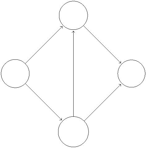

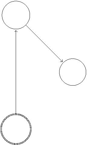


(c) Call a vertex with excess maximal if none of its descendants have excess. (Every highest vertex with
excess is maximal — do you see why? — but the converse need not hold.) For such a vertex, define
φ(v) = max{K − D(v) + 1, 0},
where K is a parameter to be chosen in part (i). For the other vertices, define φ(v) = 0. Define
X
Φ =
φ(v).
v∈V
Prove that a non-saturating push, from a highest vertex v with positive excess, cannot increase Φ.
Moreover, such a push strictly decreases Φ if D(v) ≤ K.
(d) Prove that changing a vertex’s successor from NULL to a non-NULL value cannot increase Φ.
(e) Prove that each relabel increases Φ by at most K.
[Hint: before a relabel at v, v has out-degree 0 in Sf . After the re-label, it has in-degree 0. Can this
create new maximal vertices? And how do the different D(w)’s change?]
(f) Prove that each saturating push increases Φ by at most K.
(g) A phase is a maximal sequence of operations such that the maximum height of a vertex with excess
remains unchanged. (The set of such vertices can change.) Prove that there are O(n2) phases.
(h) Arguing as in Lecture #3 shows that each phase performs at most n non-saturating pushes (why?), but
we want to beat the O(n3) bound. Suppose that a phase performs at least
Show that at least half of these strictly decrease Φ.
2n
K
non-saturating pushes.
[Hint: prove that if a phase does a non-saturating push at both v and w during a phase, then v and
w share no descendants during the phase. How many such vertices can there be with more than K
descendants?]
n3
K
(i) Prove a bound of O( + nmK) on the total number of non-saturating pushes across all phases.
√
Choose K so that the bound simplifies to O(n2 m).
Problem 6
Suppose we are given an array A[1..m][1..n] of non-negative real numbers. We want to round A to an integer
matrix, by replacing each entry x in A with either bxc or dxe, without changing the sum of entries in any
row or column of A. (Assume that all row and column sums of A are integral.) For example:
1
3
7
.2 3.4 2.4
.9 2.1
.9 1.6 0.5
1
4
8
4
4
1
2
2
1
4
→
(a) Describe and analyze an efficient algorithm that either rounds A in this fashion, or reports correctly
that no such rounding is possible.
[
Hint: don’t solve the problem from scratch, use a reduction instead.]
(b) Prove that such a rounding is guaranteed to exist.
5


CS261: Problem Set #2
Due by 11:59 PM on Tuesday, February 9, 2016
Instructions:
(1) Form a group of 1-3 students. You should turn in only one write-up for your entire group.
(2) Submission instructions: We are using Gradescope for the homework submissions. Go to www.gradescope.com
to either login or create a new account. Use the course code 9B3BEM to register for CS261. Only one
group member needs to submit the assignment. When submitting, please remember to add all group
member names in Gradescope.
(3) Please type your solutions if possible and we encourage you to use the LaTeX template provided on
the course home page.
(4) Write convincingly but not excessively.
(5) Some of these problems are difficult, so your group may not solve them all to completion. In this case,
you can write up what you’ve got (subject to (3), above): partial proofs, lemmas, high-level ideas,
counterexamples, and so on.
(6) Except where otherwise noted, you may refer to the course lecture notes only. You can also review any
relevant materials from your undergraduate algorithms course.
(7) You can discuss the problems verbally at a high level with other groups. And of course, you are
encouraged to contact the course staff (via Piazza or office hours) for additional help.
(8) If you discuss solution approaches with anyone outside of your group, you must list their names on the
front page of your write-up.
(9) Refer to the course Web page for the late day policy.
Problem 7
A vertex cover of an undirected graph (V, E) is a subset S ⊆ V such that, for every edge e ∈ E, at least one
of e’s endpoints lies in S.1
(a) Prove that in every graph, the minimum size of a vertex cover is at least the size of a maximum
matching.
(b) Give a non-bipartite graph in which the minimum size of a vertex cover is strictly bigger than the size
of a maximum matching.
(c) Prove that the problem of computing a minimum-cardinality vertex cover can be solved in polynomial
time in bipartite graphs.2
[
Hint: reduction to maximum flow.]
(d) Prove that in every bipartite graph, the minimum size of a vertex cover equals the size of a maximum
matching.
1
2
Yes, the problem is confusingly named.
In general graphs, the problem turns out to be NP-hard (you don’t need to prove this).
1

Problem 8
This problem considers the special case of maximum flow instances where edges have integral capacities and
also
(*) for every vertex v other than s and t, either (i) there is at most one edge entering v, and this edge
(if it exists) has capacity 1; or (ii) there is at most one edge exiting v, and this edge (if it exists) has
capacity 1.
Your tasks:
√
(a) Prove that the maximum flow problem can be solved in O(m n) time in networks that satisfy (*).
(As always, m is the number of edges and n is the number of vertices.)
[
Hint: proceed as in Problem 4, but prove a stronger version of part (a) of that problem.]
√
(b) Prove that the maximum bipartite matching problem can be solved in O(m n) time.
[
Hint: examine the reduction in Lecture #4.]
Problem 9
This problem considers approximation algorithms for graph matching problems.
(a) For the maximum-cardinality matching problem in bipartite graphs, prove that for every constant
ꢀ > 0, there is an O(m)-time algorithm that computes a matching with size at most ꢀn less than the
maximum possible (where n is the number of vertices). (The hidden constant in the big-oh notation
1
can depend on .)
ꢀ
[
Hint: ideas from Problem 8(b) should be useful.]
(b) Now consider non-bipartite graphs where each edge e has a real-valued weight we. Recall the greedy
algorithm from Lecture #6:
Greedy Matching Algorithm
sort and rename the edges E = {1, 2, . . . , m} so that w ≥ w ≥ · · · w
1
2
m
M = ∅
for i = 1 to m do
if w > 0 and e shares no endpoint with edges in M then
i
i
add ei to M
How fast can you implement this algorithm?
(c) Prove that the greedy algorithm always outputs a matching with total weight at least 50% times that
of the maximum possible.
[Hint: if the greedy algorithm adds an edge e to M, how many edges in the optimal matching can this
edge “block”? How do the weights of the blocked edges compare to that of e?]
Problem 10
This problem concerns running time optimizations to the Hungarian algorithm for computing minimum-cost
perfect bipartite matchings (Lecture #5). Recall the O(mn2) running time analysis from lecture: there are
at most n augmentation steps, at most n price update steps between two augmentation steps, and each
iteration can be implemented in O(m) time.
2


(a) By a phase, we mean a maximal sequence of price update iterations (between two augmentation
iterations). The naive implementation in lecture regrows the search tree from scratch after each price
update in a phase, spending O(m) time on this for each of up to n iterations. Show how to reuse work
from previous iterations so that the total amount of work done searching for good paths, in total over
all iterations in the phase, is only O(m).
[
Hint: compare to Problem 2(a).]
(b) The other non-trivial work in a price update phase is computing the value of ∆ (the magnitude of the
update). This is easy to do in O(m) time per iteration. Explain how to maintain a heap data structure
so that the total time spent computing ∆ over all iterations in the phase is only O(m log n). Be sure
to explain what heap operations you perform while growing the search tree and when executing a price
update.
[
This yields an O(mn log n) time implementation of the Hungarian algorithm.]
Problem 11
In the minimum-cost flow problem, the input is a directed graph G = (V, E), a source s ∈ V , a sink t ∈ V ,
a target flow value d, and a capacity u ≥ 0 and cost c ∈ R for each edge e ∈ E. The goal is to compute
e
sending d units from s to t with the minimum-possible cost
e
P
a flow {f }
c f . (If there is no such
e
flow, the algorithm should correctly report this fact.)
e∈E
e∈E
e
e
Given a min-cost flow instance and a feasible flow f with value d, the corresponding residual network G
f
is defined as follows. The vertex set remains V . For every edge (v, w) ∈ E with f < uvw, there is an edge
vw
(v, w) in G with cost c and residual capacity u − f . For every edge (v, w) ∈ E with f > 0, there is a
f
e
e
e
vw
reverse edge (w, v) in G with the cost −c and residual capacity f .
f
A negative cycle of G is a directed cycle C of G such that the sum of the edge costs in C is negative.
e
e
f
f
(E.g., v → w → x → y → v, with cvw = 2, cwx = −1, cxy = 3, and cyv = −5.)
(a) Prove that if the residual network Gf of a flow f has a negative cycle, then f is not a minimum-cost
flow.
(b) Prove that if the residual network Gf of a flow f has no negative cycles, then f is a minimum-cost
flow.
[Hint: look to the proof of the minimum-cost bipartite matching optimality conditions (Lecture #5)
for inspiration.]
(c) Give a polynomial-time algorithm that, given a residual network Gf , either returns a negative cycle or
correctly reports that no negative cycle exists.
[Hint: feel free to use an algorithm from CS161. Be clear about which properties of the algorithm
you’re using.]
(d) Assume that all edge costs and capacities are integers with magnitude at most M. Give an algorithm
that is guaranteed to terminate with a minimum-cost flow and has running time polynomial in n = |V |,
m = |E|, and M.3
[
Hint: what would the analog of Ford-Fulkerson be?]
Problem 12
The goal of this problem is to revisit two problems you studied in CS161 — the minimum spanning tree
and shortest path problems — and to prove the optimality of Kruskal’s and Dijkstra’s algorithms via the
complementary slackness conditions of judiciously chosen linear programs.
3
Thus this algorithm is only “pseudo-polynomial.” A polynomial algorithm would run in time polynomial in n, m, and
log M. Such algorithms can be derived for the minimum-cost flow problem using additional ideas.
3

(a) For convenience, we consider the maximum spanning tree problem (equivalent to the minimum spanning
tree problem, after multiplying everything by -1). Consider a connected undirected graph G = (V, E)
in which each edge e has a weight we.
For a subset F ⊆ E, let κ(F) denote the number of connected components in the subgraph (V, F).
Prove that the spanning trees of G are in an objective function-preserving one-to-one correspondence
with the 0-1 feasible solutions of the following linear program (with decision variables {xe}e∈E):
X
max
wexe
e∈E
subject to
X
xe ≤ |V | − κ(F)
xe = |V | − 1
for all F ⊆ E
e∈F
X
e∈E
xe ≥ 0
for all e ∈ E.
(While this linear program has a huge number of constraints, we are using it purely for the analysis of
Kruskal’s algorithm.)
(b) What is the dual of this linear program?
(c) What are the complementary slackness conditions?
(d) Recall that Kruskal’s algorithm, adapted to the current maximization setting, works as follows: do a
single pass over the edges from the highest weight to lowest weight (breaking ties arbitrarily), adding
an edge to the solution-so-far if and only if it creates no cycle with previously chosen edges. Prove that
the corresponding solution to the linear program in (a) is in fact an optimal solution to that linear
program, by exhibiting a feasible solution to the dual program in (b) such that the complementary
slackness conditions hold.4
[
E that comprise the i edges with the largest weights (for some i).]
Hint: for the dual variables of the form y , it is enough to use only those that correspond to subsets F ⊆
F
(e) Now consider the problem of computing a shortest path from s to t in a directed graph G = (V, E)
with a nonnegative cost c on each edge e ∈ E. Prove that every simple s-t path of G corresponds to
e
a 0-1 feasible solution of the following linear program with the same objective function value:5
X
min
c x
e e
e∈E
subject to
X
xe ≥ 1
xe ≥ 0
for all S ⊆ V with s ∈ S, t ∈/ S
for all e ∈ E.
e∈δ+(S)
(Again, this huge linear program is for analysis only.)
(f) What is the dual of this linear program?
(g) What are the complementary slackness conditions?
4
You can assume without proof that Kruskal’s algorithm outputs a feasible solution (i.e., a spanning tree), and focus on
proving its optimality.
Recall that δ+(S) denotes the edges sticking out of S.
5
4

(h) Let P denote the s-t path returned by Dijkstra’s algorithm. Prove that the solution to the linear
program in (e) corresponding to P is in fact an optimal solution to that linear program, by exhibiting
a feasible solution to the dual program in (f) such that the complementary slackness conditions hold.
[Hint: it is enough to use only dual variables of the form yS for subsets S ⊆ V that comprise the first i
vertices processed by Dijkstra’s algorithm (for some i).]
5
CS261: Problem Set #3
Due by 11:59 PM on Tuesday, February 23, 2016
Instructions:
(1) Form a group of 1-3 students. You should turn in only one write-up for your entire group.
(2) Submission instructions: We are using Gradescope for the homework submissions. Go to www.gradescope.com
to either login or create a new account. Use the course code 9B3BEM to register for CS261. Only one
group member needs to submit the assignment. When submitting, please remember to add all group
member names in Gradescope.
(3) Please type your solutions if possible and we encourage you to use the LaTeX template provided on
the course home page.
(4) Write convincingly but not excessively.
(5) Some of these problems are difficult, so your group may not solve them all to completion. In this case,
you can write up what you’ve got (subject to (3), above): partial proofs, lemmas, high-level ideas,
counterexamples, and so on.
(6) Except where otherwise noted, you may refer to the course lecture notes only. You can also review any
relevant materials from your undergraduate algorithms course.
(7) You can discuss the problems verbally at a high level with other groups. And of course, you are
encouraged to contact the course staff (via Piazza or office hours) for additional help.
(8) If you discuss solution approaches with anyone outside of your group, you must list their names on the
front page of your write-up.
(9) Refer to the course Web page for the late day policy.
Problem 13
This problem fills in some gaps in our proof sketch of strong linear programming duality.
(a) For this part, assume the version of Farkas’s Lemma stated in Lecture #9, that given A ∈ Rm× and
b ∈ Rm, exactly one of the following statements holds: (i) there is an x ∈ Rn such that Ax = b and
x ≥ 0; (ii) there is a y ∈ Rm such that yT A ≥ 0 and yT b < 0.
n
Deduce from this a second version of Farkas’s Lemma, stating that for A and b as above, exactly one
of the following statements holds: (iii) there is an x ∈ Rn such that Ax ≤ b; (iv) there is a y ∈ Rm
such that y ≥ 0, yT A = 0, and yT b < 0.
[
Hint: note the similarity between (i) and (iv). Also note that if (iv) has a solution, then it has a
solution with yT b = −1. ]
(b) Use the second version of Farkas’s Lemma to prove the following version of strong LP duality: if the
linear programs
max cT x
subject to
Ax ≤ b
1
with x unrestricted, and
min bT y
subject to
AT y = c, y ≥ 0
are both feasible, then they have equal optimal objective function values.
[
Hint: weak duality is easy to prove directly. For strong duality, let γ∗ denote the optimal objective
function value of the dual linear program. Add the constraint cT x ≥ γ to the primal linear program
∗
and use Farkas’s Lemma to show that the feasible region is non-empty.]
Problem 14
Recall the multicommodity flow problem from Exercise 17. Recall the input consists of a directed graph
G = (V, E), k “commodities” or source-sink pairs (s , t ), . . . , (s , t ), and a positive capacity u for each
1
1
k
k
e
edge.
Consider also the multicut problem, where the input is the same as in the multicommodity flow problem,
and feasible solutions are subsets F ⊆ E of edges such that, for every commodity (s , t ), there is no s -t
i
i
i
i
path in G = (V, E \ F). (Assume that s and t are distinct for each i.) The value of a multicut F is just
P
(a) Formulate the multicommodity flow problem as a linear program with one decision variable for each
path P that travels from a source s to the corresponding sink t . Aside from nonnegativity constraints,
i
i
the total capacity
u .
e
e∈F
i
i
there should be only be m constraints (one per edge).
[
Note: this is a different linear programming formulation than the one asked for in Exercise 21.]
(b) Take the dual of the linear program in (a). Prove that every optimal 0-1 solution of this dual —
i.e., among all feasible solutions that assign each decision variable the value 0 or 1, one of minimum
objective function value — is the characteristic vector of a minimum-value multicut.
(c) Show by example that the optimal solution to this dual linear program can have objective function
value strictly smaller than that of every 0-1 feasible solution. In light of your example, explain a sense
in which there is no max-flow/min-cut theorem for multicommodity flows and multicuts.
Problem 15
This problem gives a linear-time (!) randomized algorithm for solving linear programs that have a large
number m of constraints and a small number n of decision variables. (The constant in the linear-time
guarantee O(m) will depend exponentially on n.)
Consider a linear program of the form
max cT x
subject to
Ax ≤ b.
For simplicity, assume that the linear program is feasible with a bounded feasible region, and let M be large
enough that |x | < M for every coordinate of every feasible solution. Assume also that the linear program
j
is “non-degenerate,” in the sense that no feasible point satisfies more than n constraints with equality. For
example, in the plane (two decision variables), this just means that there does not exist three different
constraints (i.e., halfplanes) whose boundaries meet at a common point. Finally, assume that the linear
program has a unique optimal solution.1
Let C = {1, 2, . . . , m} denote the set of constraints of the linear program. Let B denote additional
constraints asserting that −M ≤ x ≤ M for every j. The high-level idea of the algorithm is: (i) drop a
j
1
All of these simplifying assumptions can be removed without affecting the asymptotic running time; we leave the details to
the interested reader.
2

random constraint and recursively compute the optimal solution x∗ of the smaller linear program; (ii) if x∗
∗
is feasible for the original linear program, return it; (iii) else, if x violates the constraint a x
change this inequality to an equality and recursively solve the resulting linear program.
T
≤
bi, then
i
More precisely, consider the following recursive algorithm with two arguments. The first argument C1 is
a subset of inequality constraints that must be satisfied (initially, equal to C). The second argument is a
subset C of constraints that must be satisfied with equality (initially, ∅). The responsibility of a recursive call
2
is to return a point maximizing cT x over all points that satisfy all the constraints of C ∪ B (as inequalities)
1
and also those of C (as equations).
2
Linear-Time Linear Programming
Input: two disjoint subsets C , C ⊆ C of constraints
1
2
Base case #1: if |C2| = n, return the unique point that satisfies every constraint
of C2 with equality
Base case #2: if |C | + |C | = n, return the point that maximizes cT x subject to
1
2
aT x ≤ b for every i ∈ C , aT x = b for every i ∈ C , and the constraints in B
i
i
1
i
i
2
Recursive step:
choose i ∈ C uniformly at random
1
recurse with the sets C \ {i} and C to obtain a point x
∗
1
2
if aT x
∗
≤
b then
i
i
∗
return x
else
recurse with the sets C \ {i} and C ∪ {i}, and return the result
1
2
(a) Prove that this algorithm terminates with the optimal solution x∗ of the original linear program.
Hint: be sure to explain why, in the “else” case, it’s OK to recurse with the ith constraint set to an
[
equation.]
(b) Let T(m, s) denote the expected number of recursive calls made by the algorithm to solve an instance
with |C | = m and |C | = s (with the number n of variables fixed). Prove that T satisfies the following
1
recurrence:
2
ꢀ
1
if s = n or m + s = n
T(m 1, s + 1) otherwise.
T(m, s) =
T(m − 1, s) +
n−s ·
−
m
[
Hint: you should use the non-degeneracy assumption in this part.]
(c) Prove that T(m, 0) ≤ n! · m.
[
induction on m and δ.]
Hint: it might be easiest to make the variable substitution δ = n − s and proceed by simultaneous
(d) Conclude that, for every fixed constant n, the algorithm above can be implemented so that the expected
running time is O(m) (where the hidden constant can depend arbitrarily on n).
3


Problem 16
This problem considers a variant of the online decision-making problem. There are n “experts,” where n is
a power of 2.
Combining Expert Advice
At each time step t = 1, 2, . . . , T:
each expert offers a prediction of the realization of a binary event (e.g., whether a
stock will go up or down)
a decision-maker picks a probability distribution pt over the possible realizations 0
and 1 of the event
the actual realization rt ∈ {0, 1} of the event is revealed
a 0 or 1 is chosen according to the distribution pt, and a mistake occurs whenever
it is different from rt
You are promised that there is at least one omniscient expert who makes a correct prediction at every time
step.
(a) Prove that the minimum worst-case number of mistakes that a deterministic algorithm can make is
precisely log2 n.
(b) Prove that the minimum worst-case expected number of mistakes that a randomized algorithm can
1
make is precisely log2 n.
2
Problem 17
In Lecture #11 we saw that the follow-the-leader (FTL) algorithm, and more generally every deterministic
algorithm, can have regret that grows linearly with T. This problem outlines a randomized variant of
FTL, the follow-the-perturbed-leader (FTPL) algorithm, with worst-case regret comparable to that of the
multiplicative weights algorithm. In the description of FTPL, we define each probability distribution pt over
actions implicitly through a randomized subroutine.
Follow-the-Perturbed-Leader (FTPL) Algorithm
for each action a ∈ A do
independently sample a geometric random variable with parameter η,2 denoted by
Xa
for each time step t = 1, 2, . . . , T do
choose the action a that maximizes the perturbed cumulative reward
t−1
P
For convenience, assume that, at every time step t, there is no pair of actions whose (unperturbed) cumulative
rewards-so-far differ by an integer.
Xa +
ru(a) so far
u=1
(a) Prove that, at each time step t = 1, 2, . . . , T, with probability at least 1 − η, the largest perturbed
cumulative reward of an action prior to t is more than 1 larger than the second-largest such perturbed
reward.
∗
[
Hint: Sample the X ’s gradually by flipping coins only as needed, pausing once the action a with
a
largest perturbed cumulative reward is identified. Resuming, only Xa∗ is not yet fully determined.
What can you say if the next coin flip comes up “tails?”]
2
Equivalently, when repeatedly flipping a coin that comes up “heads” with probability η, count the number of flips up to
and including the first “heads.”
4


(b) As a thought experiment, consider the (unimplementable) algorithm that, at each time step t, picks
u
P
t
u=1
the action that maximizes the perturbed cumulative reward Xa +
r (a) over a ∈ A, taking into
account the current reward vector. Prove that the regret of this algorithm is at most maxa∈A X .
Hint: Consider first the special case where Xa = 0 for all a. Iteratively transform the action sequence
that always selects the best action in hindsight to the sequence chosen by the proposed algorithm. Work
a
[
backward from time T, showing that the reward only increases with each step of the transformation.]
(c) Prove that E[max
Xa] ≤ bη−1 ln n, where n is the number of actions and b > 0 is a constant
a∈A
independent of η and n.
Hint: use the definition of a geometric random variable and remind yourself about “the union bound.”]
(d) Prove that, for a suitable choice of η, the worst-case expected regret of the FTPL algorithm is at
[
√
most b T ln n, where b > 0 is a constant independent of n and T.
Problem 18
In this problem we’ll show that there is no online algorithm for the online bipartite matching problem with
1
competitive ratio better than 1 −
≈
63.2%.
e
Consider the following probability distribution over online bipartite matching instances. There are n
left-hand side vertices L, which are known up front. Let π be an ordering of L, chosen uniformly at random.
The n vertices of the right-hand side R arrive one by one, with the ith vertex of R connected to the last
n − i + 1 vertices of L (according to the random ordering π).
(a) Explain why OP T = n for every such instance.
(b) Consider an arbitrary deterministic online algorithm A. Prove that for every i ∈ {1, 2, . . . , n}, the
probability (over the choice of π) that A matches the ith vertex of L (according to π) is at most
i
X
1
min
, 1
.
n − j + 1
j=1
[
Hint: for example, in the first iteration, assume that A matches the first vertex of R to the vertex
v ∈ L. Note that A must make this decision without knowing π. What can you say if v does not
happen to be the first vertex of π?]
(c) Prove that for every deterministic online algorithm A, the expected (over π) size of the matching
produced by A is at most
Xn
X
i
1
min
, 1
,
(1)
n − j + 1
i=1
j=1
and prove that (1) approaches n(1 − ) as n
1
e
→ ∞
.
P
d
1
[
Hint: for the second part, recall that
≈ ln d (up to an additive constant less than 1). For what
j=1 j
value of i is the inner sum roughly equal to 1?]
(d) Extend (c) to randomized online algorithms A, where the expectation is now over both π and the
internal coin flips of A.
[Hint: use the fact that a randomized online algorithm is a probability distribution over deterministic
online algorithms (as flipping all of A’s coins in advance yields a deterministic algorithm).]
(e) Prove that for every ꢀ > 0 and (possibly randomized) online bipartite matching algorithm A, there
exists an input such that the expected (over A’s coin flips) size of A’s output is no more than 1− +ꢀ
1
e
times that of an optimal solution.
5


CS261: Problem Set #4
Due by 11:59 PM on Tuesday, March 8, 2016
Instructions:
(1) Form a group of 1-3 students. You should turn in only one write-up for your entire group.
(2) Submission instructions: We are using Gradescope for the homework submissions. Go to www.gradescope.com
to either login or create a new account. Use the course code 9B3BEM to register for CS261. Only one
group member needs to submit the assignment. When submitting, please remember to add all group
member names in Gradescope.
(3) Please type your solutions if possible and we encourage you to use the LaTeX template provided on
the course home page.
(4) Write convincingly but not excessively.
(5) Some of these problems are difficult, so your group may not solve them all to completion. In this case,
you can write up what you’ve got (subject to (3), above): partial proofs, lemmas, high-level ideas,
counterexamples, and so on.
(6) Except where otherwise noted, you may refer to the course lecture notes only. You can also review any
relevant materials from your undergraduate algorithms course.
(7) You can discuss the problems verbally at a high level with other groups. And of course, you are
encouraged to contact the course staff (via Piazza or office hours) for additional help.
(8) If you discuss solution approaches with anyone outside of your group, you must list their names on the
front page of your write-up.
(9) Refer to the course Web page for the late day policy.
Problem 19
This problem considers randomized algorithms for the online (integral) bipartite matching problem (as in
Lecture #14).
(a) Consider the following algorithm: when a new vertex w ∈ R arrives, among the unmatched neighbors
of w (if any), choose one uniformly at random to match to w.
Prove that the competitive ratio of this algorithm is strictly smaller than 1 − .
1
e
(b) The remaining parts consider the following algorithm: before any vertices of R arrive, independently
pick a number y uniformly at random from [0, 1] for each vertex v ∈ L. Then, when a new vertex
v
w ∈ R arrives, match w to its unmatched neighbor with the smallest y-value (or to no one if all its
neighbors are already matched).
For the analysis, when v and w are matched, define q = g(y ) and q = 1 − g(yv), where g(y) = ey−
1
v
v
w
is the same function used in Lecture #14.
P
Prove that with probability 1, at the end of the algorithm,
matching.
qv equals the size of the computed
v∈L∪R
1

(c) Fix an edge (v, w) in the final graph. Condition on the choice of y for every vertex x ∈ L ∪ R \ {v}
x
other than v; q remains random. As a thought experiment, suppose we re-run the online algorithm
v
from scratch with v deleted (the rest of the input and the y-values stay the same), and let t ∈ L denote
the vertex to which w is matched (if any).
R
Hint: prove that v is matched (in the online algorithm with the original input, not in the thought
yt
Prove that the conditional expectation of q (given q for all x ∈ L ∪ R \ {v}) is at least
g(z)dz.
v
x
0
(If t does not exist, interpret y as 1.)
t
[
experiment) whenever y < y . Conditioned on this event, what is the distribution of y ?]
v
t
v
(d) Prove that, conditioned on q for all x ∈ L ∪ R \ {v}, q ≥ 1 − g(y ).
x
w
t
[
Hint: prove that w is always matched (in the online algorithm with the original input) to a vertex
with y-value at most yt.]
(e) Prove that the randomized algorithm in (b) is (1 − )-competitive, meaning that for every input, the
1
e
expected value of the computed matching (over the algorithm’s coin flips) is at least 1 − times the
1
e
size of a maximum matching.
[
Hint: use the expectation of the q-values to define a feasible dual solution.]
Problem 20
A set function f : 2U → R+ is monotone if f(S) ≤ f(T) whenever S ⊆ T ⊆ U. Such a function is submodular
if it has diminishing returns: whenever S ⊆ T ⊆ U and i ∈/ T, then
f(T ∪ {i}) − f(T) ≤ f(S ∪ {i}) − f(S).
(1)
We consider the problem of, given a function f and a budget k, computing1
max f(S).
S⊆U:|S|=k
(2)
(a) Prove that set coverage problem (Lecture #15) is a special case of this problem.
(b) Let G = (V, E) be a directed graph and p ∈ [0, 1] a parameter. Recall the cascade model from Lecture
#
15:
•
Initially the vertices in some set S are “active,” all other vertices are “inactive.” Every edge is
initially “undetermined.”
•
While there is an active vertex v and an undetermined edge (v, w):
–
–
with probability p, edge (v, w) is marked “active,” otherwise it is marked “inactive;”
if (v, w) is active and w is inactive, then mark w as active.
Let f(S) denote the expected number of active vertices at the conclusion of the cascade, given that the
vertices of S are active at the beginning. (The expectation is over the coin flips made for the edges.)
Prove that f is monotone and submodular.
[
Hint: prove that the condition (1) is preserved under convex combinations.]
(c) Let f be a monotone submodular function. Define the greedy algorithm in the obvious way — at each
of k iterations, add to S the element that increases f the most. Suppose at some iteration the current
greedy solution is S and it decides to add i to S. Prove that
1
f(S ∪ {i}) − f(S) ≥ (OP T − f(S)) ,
k
where OP T is the optimal value in (2).
[Hint: If you added every element in the optimal solution to S, where would you end up? Then use
submodularity.]
1
Don’t worry about how f is represented in the input. We assume that it is possible to compute f(S) from S in a reasonable
amount of time.
2


(d) Prove that for every monotone submodular function f, the greedy algorithm is a (1− )-approximation
1
e
algorithm.
Problem 21
This problem considers the “{1, 2}” special case of the asymmetric traveling salesman problem (ATSP). The
input is a complete directed graph G = (V, E), with all n(n − 1) directed edges present, where each edge e
has a cost c that is either 1 or 2. Note that the triangle inequality holds in every such graph.
e
(a) Explain why the {1, 2} special case of ATSP is NP-hard.
(b) Explain why it’s trivial to obtain a polynomial-time 2-approximation algorithm for the {1, 2} special
case of ATSP.
(c) This part considers a useful relaxation of the ATSP problem. A cycle cover of a directed graph
G = (V, E) is a collection C , . . . , C of simple directed cycles, each with at least two edges, such that
1
k
every vertex of G belongs to exactly one of the cycles. (A traveling salesman tour is the special case
where k = 1.) Prove that given a directed graph with edge costs, a cycle cover with minimum total
cost can be computed in polynomial time.
[
Hint: bipartite matching.]
(d) Using (c) as a subroutine, give a -approximation algorithm for the 1, 2 special case of the ATSP
{
3
2
}
problem.
Problem 22
This problem gives an application of randomized linear programming rounding in approximation algorithms.
In the uniform labeling problem, we are given an undirected graph G = (V, E), costs c ≥ 0 for all edges
e
e ∈ E, and a set L of labels that can be assigned to the vertices of V . There is a non-negative cost ci ≥ 0 for
v
assigning label i ∈ L to vertex v ∈ V , and the edge cost c is incurred if and only if e’s endpoints are given
e
distinct labels. The goal of the problem is to assign each vertex a label so as to minimize the total cost.2
(a) Prove that the following is a linear programming relaxation of the problem:
X
X
X X
1
2
i
i
i
min
ce
z +
c x
v
e
v
e∈E
i∈L
v∈V i∈L
subject to
X
i
x = 1
for all v ∈ V
v
i∈L
i
i
i
z ≥ x − x
for all e = (u, v) ∈ E and i ∈ L
for all e = (u, v) ∈ E and i ∈ L
for all e ∈ E and i ∈ L
e
u
v
i
i
v
i
u
z ≥ x − x
e
i
e
z ≥ 0
i
v
x ≥ 0
Specifically, prove that for every feasible solution to the uniform labeling problem, there is a corre-
for all v ∈ V and i ∈ L.
sponding 0-1 feasible solution to this linear program that has the same objective function value.
2
The motivation for the problem comes from image segmentation, generalizing the foreground-background segmentation
problem discussed in Lecture #4.
3


(b) Consider now the following algorithm. First, the algorithm solves the linear programming relaxation
above. The algorithm then proceeds in phases. In each phase, it picks a label i ∈ L uniformly at
random, and independently a number α ∈ [0, 1] uniformly at random. For each vertex v ∈ V that has
not yet been assigned a label, if α ≤ xi , then we assign v the label i (otherwise it remains unassigned).
v
To begin the analysis of this randomized rounding algorithm, consider the start of a phase and suppose
that the vertex v ∈ V has not yet been assigned a label. Prove that (i) the probability that v is
assigned the label i in the current phase is exactly xi /|L|; and (ii) the probability that it is assigned
v
some label in the current phase is exactly 1/|L|.
(c) Prove that the algorithm assigns the label i ∈ L to the vertex v ∈ V with probability exactly xiv.
(d) We say that an edge e is separated by a phase if both endpoints were not assigned prior to the phase,
and exactly one of the endpoints is assigned a label in this phase. Prove that, conditioned on neither
endpoint being assigned yet, the probability that an edge e is separated by a given phase is at most
P
1
L|
i
z .
|
i∈L
e
(e) Prove that, for every edge e, the probability that the algorithm assigns different labels to e’s endpoints
zi.
P
relate the probability of this to the quantity
is at most
i∈L
Hint: it might help to identify a sufficient condition for an edge e = (u, v) to not be separated, and to
e
[
P
min{xi , xi }.]
i∈L
u
v
(f) Prove that the expected cost of the solution returned by the algorithm is at most twice the cost of an
optimal solution.
Problem 23
This problem explores local search as a technique for designing good approximation algorithms.
(a) In the Max k-Cut problem, the input is an undirected graph G = (V, E) and a nonnegative weight we
for each edge, and the goal is to partition V into at most k sets such that the sum of the weights of
the cut edges — edges with endpoints in different sets of the partition — is as large as possible. The
obvious local search algorithm for the problem is:
1
2
. Initialize (S , . . . , S ) to an arbitrary partition of V .
1
k
. While there exists an improving move:
[
increases the objective function.]
An improving move is a vertex v ∈ S and a set S such that moving v from S to S strictly
i
j
i
j
(a) Choose an arbitrary improving move and execute it — move the vertex v from S to S .
j
i
Since each iteration increases the objective function value, this algorithm cannot cycle and eventually
terminates, at a “local maximum.”
Prove that this local search algorithm is guaranteed to terminate at a solution with objective function
k−1
value at least
times the maximum possible.
k
[Hint: prove the statement first for k = 2; your argument should generalize easily. Also, you might
find it easier to prove the stronger statement that the algorithm’s final partition has objective function
k−1
value at least
times the sum of all the edge weights.]
k
(b) Recall the uniform metric labeling problem from Problem 22. We now give an equally good approxi-
mation algorithm based on local search.
Our local search algorithm uses the following local move. Given a current assignment of labels to
vertices in V , it picks some label i ∈ L and considers the minimum-cost i-expansion of the label i; that
is, it considers the minimum-cost assignment of labels to vertices in V in which each vertex either keeps
its current label or is relabeled with label i (note that all vertices currently with label i do not change
their label). If the cost of the labeling from the i-expansion is cheaper than the current labeling, then
4

we switch to the labeling from the i-expansion. We continue until we find a locally optimal solution;
that is, an assignment of labels to vertices such that every i-expansion can only increase the cost of
the current assignment.
Give a polynomial-time algorithm that computes an improving i-expansion, or correctly decides that
no such improving move exists.
[
Hint: recall Lecture #4.]
(c) Prove that the local search algorithm in (b) is guaranteed to terminate at an assignment with cost at
most twice the minimum possible.
[Hint: the optimal solution suggests some local moves. By assumption, these are not improving. What
do these inequalities imply about the overall cost of the local minimum?]
Problem 24
This problem considers a natural clustering problem, where it’s relatively easy to obtain a good approximation
algorithm and a matching hardness of approximation bound.
The input to the metric k-center problem is the same as that in the metric TSP problem — a complete
undirected graph G = (V, E) where each edge e has a nonnegative cost ce, and the edge costs satisfy the
triangle inequality (cuv + cvw ≥ cuw for all u, v, w ∈ V ). Also given is a parameter k. Feasible solutions
correspond to choices of k centers, meaning subsets S ⊆ V of size k. The objective function is to minimize
the furthest distance from a point to its nearest center:
min max min c .
sv
S⊆V : |S|=k v∈V s∈S
(3)
We’ll also refer to the well-known NP-complete Dominating Set problem, where given an undirected
graph G and a parameter k, the goal is to decide whether or not G has a dominating set of size at most k.3
(a) (No need to hand in.) Let OPT denote the optimal objective function value (3). Observe that OPT
n
ꢀ
ꢁ
equals the cost ce of some edge, which immediately narrows down its possible values to a set of
different possibilities (where n = |V |).
2
(b) Given an instance G to the metric k-center problem, let GD denote the graph with vertices V and
with an edge (u, v) if and only if the edge cost cuv in G is at most 2D. Prove that if we can efficiently
compute a dominating set of size at most k in GD, then we can efficiently compute a solution to the
k-center instance that has objective function value at most 2D.
(c) Prove that the following greedy algorithm computes a dominating set in GOP T with size at most k:
–
–
S = ∅
While S is not a dominating set in G
:
OP T
∗
Let v be a vertex that is not in S and has no neighbor in S — there must be one, by the
definition of a dominating set — and add v so S.
[Hint: the optimal k-center solution partitions the vertex set V into k “clusters,” where the ith group
consists of those vertices for which the ith center is the closest center. Argue that the algorithm above
never picks two different vertices from the same cluster.]
(d) Put (a)–(c) together to obtain a 2-approximation algorithm for the metric k-center problem. (The
running time of your algorithm should be polynomial in both n and k.)
(e) Using a reduction from the Dominating Set problem, prove that for every ꢀ > 0, there is no (2 − ꢀ)-
approximation algorithm for the metric k-center problem, unless P = NP.
[
Hint: look to our reduction to TSP (Lecture #16) for inspiration.]
3
A dominating set is a subset S ⊆ V of vertices such that every vertex v ∈ V either belongs to S or has a neighbor in S.
5

