经典卷积架构的PyTorch实现：MobileNet V2

MobileNet V2

MobileNet V2在MobileNet V1的基础上，引入了线性瓶颈(Linear Bottlenecks)和倒残差结构(Inverted residuals)。

Linear Bottlenecks

作者认为，非线性的激活函数，比如ReLU，会导致信息的丢失。

具体地，作者将一个二维空间的流形( manifolds)通过一个后接ReLU激活的变换矩阵，嵌入到另一个维度的空间中，然后再投影回原来的二维空间。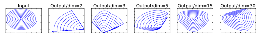

结果显示：当另一个空间的维度较低(n=2,3,5)时，还原效果很差；当另一个空间维度高一些(n=15,30)时，才能够基本还原。

但是，在接下来你会看到，这里采用的Inverted residuals中的通道数会被最后一个1x1进行压缩，也就是要将3x3卷积提取的特征进行压缩，但这样做就对应了上述实验中另一个空间维度较低时的情况，即"信息丢失"。

针对这个问题，作者提出将卷积后的激活函数设置为线性的。实验证明，该方法能够有效保留信息。具体实现时，只需去掉本来在卷积后的非线性激活函数即可。

Inverted residuals

在ResNet中，你已经见过瓶颈结构，它是一个两头粗，中间细的结构，而这里的Inverted residuals正好相反，下面来具体看一下。

仔细回想，在ResNet中，第一个1x1卷积负责降低通道数，中间的3x3卷积用于提取特征（通道数不变），第二个的1x1卷积负责升高通道数，通道数变化情况为：高-->低-->高，正好是一个瓶颈结构。

而在这里的Inverted residuals中，第一个1x1卷积负责增大通道数(低-->高)，中间的3x3卷积用于提取特征（通道数不变），第二个1x1卷积负责降低通道数(高-->低)，这与ResNet中的瓶颈结构正好相反。此时的结构类似一个纺锤体：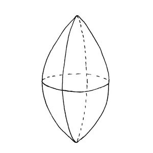

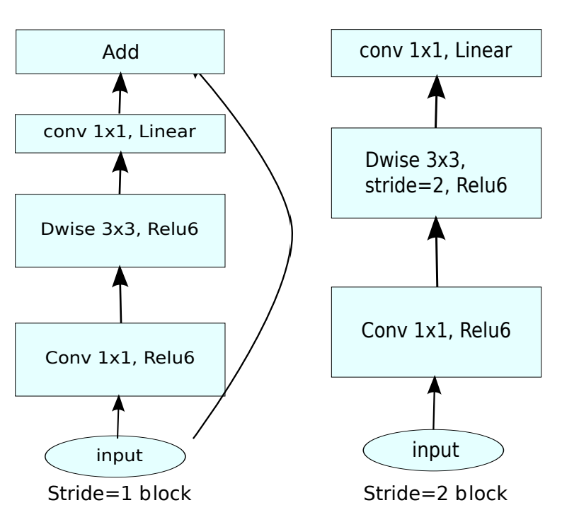
融合我们上面所讲的 Linear Bottlenecks以及Inverted residuals，就得到了MobileNet V2中的bottleneck，其具体结构如下：

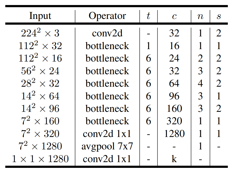
完整的MobileNetV2网络结构如下：

其中：

t：expand_ratio，即输入通道变化倍数；

c：通道数；

n：该模块重复次数；

s：stride。注意：对于n>1的情况，只有第一个重复块的的stride等于s，剩余重复块的stride均为1。

PyTorch 实现 MobileNet V2

现在来实现MobileNet V2。

首先实现网络结构图中的bottleneck：

class InvertedResidual(nn.Module):
    def __init__(self,in_channels,out_channels,stride,expand_ratio=1):
        super().__init__()
        self.stride=stride
        hidden_dim=int(in_channels*expand_ratio)# 增大（减小）通道数
        # 只有在输入与输出维度完全一致时才做跳连
        # stride=1时特征图尺寸不会改变；in_channels==out_channels，即输入输出通道数相同时，满足维度完全一致，因此可做跳连
        self.use_res_connect= self.stride==1 and in_channels==out_channels
        
        # 只有第一个bottleneck的expand_ratio=1(结构图中的t=1)，此时不需要前面的point wise conv
        if expand_ratio==1:
            self.conv=nn.Sequential(
                # depth wise conv
                nn.Conv2d(hidden_dim,hidden_dim,kernel_size=3,stride=self.stride,padding=1,groups=hidden_dim,bias=False),
                nn.BatchNorm2d(hidden_dim),# 由于expand_ratio=1，因此此时hideen_dim=in_channels
                nn.ReLU6(inplace=True),
                # point wise conv,线性激活（不加ReLU6）
                nn.Conv2d(hidden_dim,out_channels,kernel_size=1,stride=1,padding=0,groups=1,bias=False),
                nn.BatchNorm2d(out_channels)
                )
            
        # 剩余的bottlenek结构
        else:
            self.conv=nn.Sequential(
                # point wise conv
                nn.Conv2d(in_channels,hidden_dim,kernel_size=1,stride=1,padding=0,groups=1,bias=False),
                nn.BatchNorm2d(hidden_dim),
                nn.ReLU6(inplace=True),
                # depth wise conv
                nn.Conv2d(hidden_dim,hidden_dim,kernel_size=3,stride=self.stride,padding=1,groups=hidden_dim,bias=False),
                nn.BatchNorm2d(hidden_dim),
                nn.ReLU6(inplace=True),
                # point wise conv,线性激活（不加ReLU6）
                nn.Conv2d(hidden_dim,out_channels,kernel_size=1,stride=1,padding=0,groups=1,bias=False),
                nn.BatchNorm2d(out_channels)
                )
    def forward(self,x):
        if self.use_res_connect:
            return x+self.conv(x)
        else:
            return self.conv(x)

1x1 conv的stride始终固定为1，因此传入的stride仅针对3x3的depth wise conv有效：当stride=1时，特征图尺寸不变；当stride=2时，特征图尺寸减半。

stride=1时特征图尺寸不会改变；in_channels=out_channels时，输入输出通道数相同。这两个条件都满足时，输入与输出的维度完全一致，因此可做跳连，其余情况则不做。

这里的非线性激活函数统一使用了ReLU6，事实上，在MobileNet V1中就使用过ReLU6。它将原始ReLU作用后的取值限定在之间，而不是，这是为了使得模型在低精度时也能够具有较强的能力，更多细节可自行搜索。

有了bottleneck，就能够实现MobileNet V2了：

class MobileNetV2(nn.Module):
    def __init__(self,num_classes=1000,img_channel=3,width_mult=1.0):
        super().__init__()
        in_channels=32#第一个c
        last_channels=1280#最后的c
        #根据网络结构图得到如下网络配置
        inverted_residual_setting=[
            # t, c, n, s
            [1, 16, 1, 1],
            [6, 24, 2, 2],
            [6, 32, 3, 2],
            [6, 64, 4, 2],
            [6, 96, 3, 1],
            [6, 160, 3, 2],
            [6, 320, 1, 1],            
        ]
        
        #1. building first layer,网络结构图中第一行的普通conv2d
        #这里的input_channel指的是第一个bottlenek的输入通道数
        input_channel = _make_divisible(in_channels * width_mult, 4 if width_mult == 0.1 else 8)
        #print(input_channel)#32
        layers=[self.conv_3x3_bn(in_channels=img_channel,out_channels=input_channel,stride=2)]
        
        #2. building inverted residual blocks
        for t,c,n,s in inverted_residual_setting:
            output_channel = _make_divisible(c * width_mult, 4 if width_mult == 0.1 else 8)
            #print(output_channel)#每次循环依次为：32,16,24,32,64,96,160,320
            for i in range(n):
                #InvertedResidual中的参数顺序：in_channels,out_channels,stride,expand_ratio
                layers.append(InvertedResidual(input_channel,output_channel,s if i==0 else 1,t))
                input_channel=output_channel#及时更新通道数
        self.features=nn.Sequential(*layers)
        
        #3. building last several layers
        output_channel = _make_divisible(last_channels * width_mult, 4 if width_mult == 0.1 else 8) if width_mult > 1.0 else last_channels
        #print(output_channel)#1280
        #网络结构图中倒数第三行的普通conv2d
        self.conv=self.conv_1x1_bn(in_channels=input_channel,out_channels=output_channel)
        self.avgpool = nn.AdaptiveAvgPool2d((1, 1))
        self.classifier = nn.Linear(output_channel, num_classes)
        
    def conv_3x3_bn(self,in_channels,out_channels,stride):
        return nn.Sequential(
            nn.Conv2d(in_channels=in_channels,out_channels=out_channels,kernel_size=3,stride=stride,padding=1,groups=1,bias=False),
            nn.BatchNorm2d(out_channels),
            nn.ReLU6(inplace=True)
        )
    
    def conv_1x1_bn(self,in_channels,out_channels):
        return nn.Sequential(
            nn.Conv2d(in_channels=in_channels,out_channels=out_channels,kernel_size=1,stride=1,padding=0,groups=1,bias=False),
            nn.BatchNorm2d(out_channels),
            nn.ReLU6(inplace=True)
        )
    
    def forward(self,x):
        x=self.features(x)
        x=self.conv(x)
        x=self.avgpool(x)
        x=x.view(x.size(0),-1)
        x=self.classifier(x)
        return x     

上述代码首先实现了网络结构图中最开始的Conv2d，接着使用for循环实现了bottleneck的堆叠，最后实现了剩余的层(Conv2d，avgpool，Conv2d)。

其中，_make_divisible
函数实现如下：

def _make_divisible(v, divisor, min_value=None):
    if min_value is None:
        min_value = divisor
    new_v = max(min_value, int(v + divisor / 2) // divisor * divisor)
    # Make sure that round down does not go down by more than 10%.
    #确保通道数减少量不能超过10%
    if new_v < 0.9 * v:
        new_v += divisor
    return new_v

该函数的作用是将通道数调整为8或4的倍数（这里是8），以便更能利用硬件进行加速，关于这一点了解即可，这里给出一个直观的测试结果：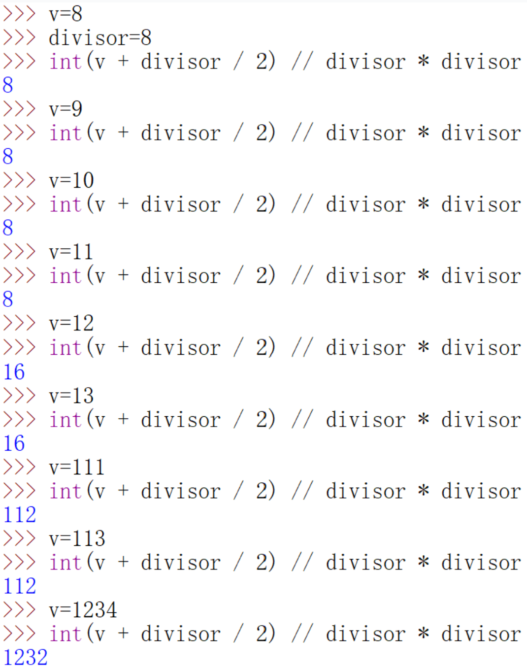

看，通道数总能够被转化为8的倍数。

最后，来测试一下刚刚实现的MobileNet V2：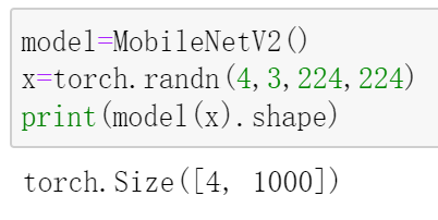

参考：

• [1] https://arxiv.org/pdf/1801.04381.pdf
• [2] https://github.com/d-li14/mobilenetv2.pytorch/blob/master/models/imagenet/mobilenetv2.py
• [3] https://www.bilibili.com/video/BV1qE411T7qZ?from=search&seid=14184470112160598991