



C
Instructor: Chandra Chekuri
Lecture date: 01/19/2010
Scribe: Alina Ene
1
Introduction and Motivation
Roughly speaking, an optimization problem has the following outline: given an instance of the
problem, find the “best” solution among all solutions to the given instance. We will be mostly
interested in discrete optimization problems where the instances and the solution set for each
instance is from a discrete set. This is in contrast to continuous optimization where the input
instance and the solution set for an instance can come from a continuous domain. Some of these
distinctions are not as clear-cut as linear programming shows.
We assume familiarity with the computational complexity classes P , NP , coNP . In this
class we are mainly interested in polynomial time solvable “combinatorial” optimization problems.
Combinatorial optimization problems are a subset of discrete optimization problems although there
is no formal definition for them. A typical problem in combinatorial optimization has a ground set
E of objects and solutions correspond to some subsets of 2E (the power set of
E
) and a typical
goal is to find either a maximum or minimum weight solution for some given weights on E. For
example, in the spanning tree problem, the ground set E is the set of edges of a graph G = (V, E)
and the solutions are subsets of E that correspond to spanning trees in G.
We will be interested in NP optimization problems – NPO problems for short. Formally, a
problem Q is a subset of Σ∗, where Σ is a finite alphabet such as binary. Each string I in Q is an
instance of Q. For a string x we use |x| to denote its length. We say that Q is an NPO problem
if the following hold:
(i) for each x ∈ Σ∗ there is a polynomial time algorithm that can check if x ∈ Q, i.e., if x is a
valid instance of Q
(ii) for each instance I there is a set sol(I) ⊂ Σ∗ such that
(a) ∀s ∈ sol(I), |s| = poly(|I|)
(b) there exists a poly-time algorithm that on input I, s correctly outputs whether s ∈ sol(I)
or not
(iii) there is a function val : Σ∗ × Σ∗ → Z s.t. val(I, s) assigns an integer to each instance I and
s ∈ sol(I) and moreover val can be computed by a poly-time algorithm.
Given an NPO problem, we say it is a minimization problem if the goal is to compute, given I ∈ Q,
arg min
val(I, s). It is a maximization problem if the goal is to compute arg max
val(I, s).
s∈sol(I)
s∈sol(I)
A natural decision problem associated with an NPO problem (say, maximization) is: given I and
integer k, is there s ∈ sol(I) s.t. val(s, I) ≥ k.
Many problems we encounter are NPO problems. Some of them can be solved in polynomial
time. It is widely believed and conjectured that P = NP , which would mean that there are
NPO problems (in particular, those whose decision versions are NP -complete) that do not have
polynomial time algorithms. Assuming P = NP , some important and useful questions are: What
problems are in P ? What characterizes problems in P ?

These are not easy questions. One insight over the years is that computation and algorithms are
difficult to understand and we are far from being able to characterize the complexity of problems.
However, in limited settings we seek to study broad classes of problems and understand some unify-
ing themes. One particular class of problems where this has been possible is the class of constraint
satisfaction problems in the Boolean domain. A result of Schaefer completely characterizes which
problems are in P and which are NP -complete. In fact, there is a nice dichotomy. However, the
non-Boolean domain is much more complicated even in this limited setting.
In the field of combinatorial optimization some unified and elegant treatment can be given via
polyhedra and the ellipsoid method. The purpose of this course is to expose you to some of these
ideas as well as outline some general problems that are known to be solvable in polynomial time.
The three ingredients in our study are
(i) polynomial time algorithms
(ii) structural results, especially via min-max characterizations of optimal solutions
(iii) polyhedral combinatorics
We will illustrate these ingredients as we go along with examples and general results. In this
introductory lecture, we discuss some known examples to highlight the view point we will take.
2
Network Flow
Given directed graph D = (V, A), two distinct nodes s, t ∈ V , and arc capacities c : A → R+, a
flow is a function f : A → R+ s.t.
P
P
(i)
f(a) =
f(a) for all v ∈ V − {s, t}
a∈δ+(v)
a∈δ−(v)
(ii) 0 ≤ f(a) ≤ c(a) for all a ∈ A
The value of f is
X
X
X
X
val(f) =
f(a) −
f(a) =
f(a) −
f(a)
a∈δ+(s)
a∈δ−(s)
a∈δ−(t)
a∈δ+(t)
The optimization problem is to maximize the flow from s to t.
An s-t cut is a partition of V into (A, B) s.t. s ∈ A, t ∈ B, and the capacity of this cut is
X
c(A, B) =
c(a)
a∈δ+(A)
Clearly, for any s-t flow f and any s-t cut (A, B)
val(f) ≤ c(A, B) ⇒ max s-t flow ≤ min s-t cut capacity
The well-known maxflow-mincut theorem of Menger and Ford-Fulkerson states that
Theorem 1 In any directed graph, the max s-t flow value is equal to the min s-t cut capacity.
Ford and Fulkerson proved the above theorem algorithmically. Although their augmenting path
algorithm is not a polynomial-time algorithm, it can be made to run in polynomial time with very
slight modifications (for example, the Edmonds-Karp modification to use the shortest augmenting
path). Moreover, the algorithm shows that there is an integer valued maximum flow whenever the
capacities are integer valued. Thus we have
Theorem 2 In any directed graph, the max s-t flow value is equal to the min s-t cut capacity.
Moreover, if c is integer valued then there is an integer valued maximum flow.
This is an example of a polynomial time (good) algorithm revealing structural properties of the
problem in terms of a min-max result and integrality of flows. Conversely, suppose we knew the
maxflow-mincut theorem but did not know any algorithmic result. Could we gain some insight?
We claim that the answer is yes. Consider the decision problem: given G, s, t, is the s-t max flow
value at least some given number k? It is easy to see that this problem is in NP since one can
give a feasible flow f of value at least k as an NP certificate1. However, using the maxflow-mincut
theorem we can also see that it is in coNP . To show that the flow value is smaller than k,
all we need to exhibit is a cut of capacity smaller than k. Therefore the min-max result shows
that the problem is in NP ∩ coNP . Most “natural” decision problems in NP ∩ coNP have
eventually been shown to have polynomial time algorithms (there are a few well-known exceptions).
Moreover, a problem in NP ∩ coNP being NP -complete or coNP -complete would imply that
NP = coNP , some thing that most believe is unlikely. Thus a min-max result implies that the
decision version is in NP ∩ coNP , strong evidence for the existence of a poly-time algorithm.
That does not imply that such an algorithm will come by easily. Examples include matchings in
general graphs and linear programming.
Finally, let us consider network flow as a special case of a linear programming problem. We can
write it as
X
X
max
f(a) −
f(a)
a∈δ+(s)
a∈δ−(s)
s.t.
f(a) −
X
X
f(a) = 0
∀v ∈ V, v = s, t
a∈δ+(v)
a∈δ−(v)
f(a) ≤ c(a)
f(a) ≥ 0
∀a ∈ A
∀a ∈ A
From the polynomial time solvability of LP, one can conclude a poly-time algorithm for network
flow. However, one can say much more. It is known that the matrix defining the above system of
inequalities is totally unimodular (TUM). From this, we have that the vertices of the polytope are
integral whenever the capacities are integral! Not only that, the dual also has integer vertices since
the objective function has integer coefficients. In fact, one can derive the maxflow-mincut theorem
from these facts about the polyhedra in question. In addition, one can derive more quite easily.
For example, we could add lower bounds on the flow
`
(a) ≤ f(a) ≤ c(a)
1We are ignoring a technicality here that the flow specification be of polynomial size in the input.

and one still obtains the fact that if there exists a flow that respects the lower/upper bounds and
, c are integer valued, then there is a corresponding integer valued flow. Same for min-cost flow
and several other variants such as circulations and transshipments.
`
3
Bipartite Matchings
Many of you have seen bipartite matchings reduced to flow. We can also treat them independently.
Let G = (X ∪ Y, E) be a bipartite graph with bipartition given by X, Y . Recall that M ⊆ E is a
matching in a graph if no vertex in G is incident to more than one edge in M.
A vertex cover in G = (V, E) is a subset of vertices S ⊆ V such that for each edge uv ∈ E, u or
v is in S. In other words, S covers all edges. We use ν(G) to indicate the cardinality of a maximum
matching in G and τ(G) for the cardinality of a minimum vertex cover in G.
Proposition 3 For every G, ν(G) ≤ τ(G).
In bipartite graphs, one has the following theorem.
Theorem 4 (Ko¨nig’s Theorem) If G is bipartite then ν(G) = τ(G).
The above proves that the max matching and min vertex problems (decision versions) in bipartite
graphs are both in NP ∩ coNP . (Note that the vertex cover problem is NP -hard in general
graphs.) We therefore expect a polynomial time algorithm for ν(G) and τ(G) in bipartite graphs. As
you know, one can reduce matching in bipartite graphs to maxflow and Ko¨nig’s theorem follows from
the maxflow-mincut theorem. One can also obtain a polynomial time augmenting path algorithm
for matching in bipartite graphs (implicitly a maxflow algorithm) that proves Ko¨nig’s theorem
algorithmically.
We now look at the polyhedral aspect. We can write a simple LP as a relaxation for the
maximum matching in a graph G.
X
max
x(e)
e∈E
X
x(e) ≤ 1
∀u ∈ V
∀e ∈ E
e∈δ(u)
x(e) ≥ 0
For bipartite graphs the above LP and its dual have integral solutions since the constraint matrix
is TUM. One can easily derive Ko¨nig’s theorem and a polynomial time algorithm from this. One
also obtains a polynomial time algorithm for weighted matching (assignment problem).
4
General Graph Matchings
The constraint matrix of the basic LP for matchings given above is not integral for general graphs,
as the following simple graph shows. Let G = K3 be the complete graph on 3 vertices. The solution
x(e) = 1/2 for each of the 3 edges in G is an optimum solution to the LP of value 3/2 while the
maximum matching in G has size 1.
The algorithmic study of general graph matchings and the polyhedral theory that was devel-
oped by Jack Edmonds in the 1960’s, and his many foundational results are the start of the field
of polyhedral combinatorics. Prior to the work of Edmonds, there was a min-max result for ν(G)
due to Berge which is based on Tutte’s necessary and sufficient condition for the existence of a
perfect matching. To explain this, for a set U ⊆ V , let o(G − U) be the number of odd cardinality
components in the graph obtained from G by removing the vertices in U.
Tutte-Berge formula
1
2
ν(G) = min (|V | + |U| − o(G − U))
U⊆V
We will prove the easy direction for now, i.e.,
1
ν(G) ≤ (|V | + |U| − o(G − U))
∀U ⊆ V
2
To see this, the number of unmatched vertices is at least o(G−U)−|U|, since each odd component
in G − U needs a vertex in U. Hence
|
V | o(G − U) − |U|
1
2
ν(G) ≤
−
≤
(|V | + |U| − o(G − U))
2
2
Corollary 5 (Tutte’s 1-factor theorem) G has a perfect matching iff ∀U ⊆ V o(G − U) ≤ |U|.
The formula shows that the decision version of matching is in NP ∩ coNP . Edmonds gave the
first polynomial time algorithms for finding a maximum cardinality matching and also more difficult
maximum weight matching problem. As a consequence of his algorithmic work, Edmonds showed
the following results on matching polytopes.
Consider the following polytope:
X
x(e) ≤ 1
x(e) ≤ b
∀v ∈ V
e∈δ(v)
X
|
U|
c
∀U, |U| odd
∀e ∈ E
2
e∈E[U]
0
≤ x(e)
Edmonds showed that the vertices of the above polytope are exactly the characteristic vectors of
the matchings of G. Observe that the polytope has an exponential number of constraints. One
can ask whether this description of the matching polytope useful. Clearly if one takes the convex
hull of the matchings of G, one obtains a polytope in RE; one can do this for any combinatorial
optimization problem and in general one gets an exponential number of inequalities. Edmonds
argued that the matching polytope is different since
(i) the inequalities are described implicitly in an uniform way
(ii) his algorithms gave a way to optimize over this polytope




At that time, no poly-time algorithm was known for solving LPs, although LP was known to be in
NP ∩coNP . In 1978, Khachiyan used the ellipsoid algorithm to show that linear programming is
in P . Very soon, Padberg-Rao, Karp-Papadimitriou, and Gro¨tschel-Lo¨vasz-Schrijver independently
realized that the ellipsoid algorithm has some very important features, and can be used to show
the polynomial-time equivalence of optimization and separation for polyhedra.
Separation Problem for Polyhedron Q
Given n (the dimension of Q), and an upper bound L on the size of the numbers defining the in-
equalities of Q, and a rational vector x ∈ Rn, output correctly either that Q x ∈ Q or a hyperplane
0
ax = b s.t. ax ≤ b ∀x ∈ Q and ax > b.
0
Optimization Problem for Polyhedron Q
Given n (the dimension of Q), and an upper bound L on the size of the numbers defining the
inequalities of Q, and a vector c ∈ Rn, output correctly one of the following: (i) Q is empty (ii)
max
cx has no finite solution (iii) a vector x∗ s.t. cx∗ = maxx∈Q cx.
x∈Q
Theorem 6 (Gro¨tschel-Lo¨vasz-Schrijver) There is a polynomial time algorithm for the separation
problem over Q iff there is a polynomial time algorithm for the optimization problem over Q.
The above consequence of the ellipsoid method had/has a substantial theoretical impact on com-
binatorial optimization. In effect, it shows that an algorithm for a combinatorial optimization
problem implies an understanding of the polytope associated with the underlying problem and
vice-versa. For example, the weighted matching algorithm of Edmonds implies that one can sep-
arate over the matching polytope. Interesting, it took until 1982 for Padberg and Rao to find
an explicit separation algorithm for the matching polytope although one is implied by the above
theorem.
References
[
[
1] J. Edmonds Paths, trees, and flowers. Canadian J. of Mathematics, 17, 449–467, 1965.
2] J. Edmonds Maximum matching and a polyhedron with 0,1 vertices. J. of Research National
Bureau of Standards Section B, 69, 73–77, 1965.
[
[
3] M. Gro¨tschel, L. Lo¨vasz and A. Schrijver. Goemetric Algorithms and Combinatorial Optimiza-
tion. Springer, 1988.
4] L.G. Khachiyan. Polynomial algorithms in linear programming. (English translation of original
Russian article). Doklady Akademii Nauk SSSR 244, 1093–1096, 1979.
[
[
5] A. Schrijver. Theory of Linear and Integer Programming (Paperback). Wiley, 1998.
6] A. Schrijver. Combinatorial Optimization: Efficiency and Polyhedra. Springer, 2003.
CS 598CSC: Combinatorial Optimization
Instructor: Chandra Chekuri
Lecture date: January 21, 2009
Scribe: Sungjin Im
1
Polyhedra and Linear Programming
In this lecture, we will cover some basic material on the structure of polyhedra and linear programming.
There is too abundant material on this topic to be covered in a few classes, so pointers will be given for
further reading. For algorithmic and computational purposes one needs to work with rational polyhedra.
Many basic results, however, are valid for both real and rational polyhedra. Therefore, to expedite our
exploration, we will not make a distinction unless necessary.
1
.1 Basics
P
Definition 1. Let x , x , ..., x be points in Rn. Let x = m λ x , where each λ ∈ R, 1 ≤ i ≤ m is a
1
2
m
i
i
i
i=1
scalar. Then, x is said to be a(n)
1
2
3
4
. Linear combination (of x , 1 ≤ i ≤ m) for arbitrary scalars λ .
i
i
P
. Affine combination if
λi = 1.
i
. Conical combination if λ ≥ 0.
i
P
. Convex combination if
λ = 1 and λ ≥ 0 (affine and also canonical).
i
i
In the following definitions and propositions, unless otherwise stated, it will be assumed that x , x , ..., x
1
2
m
are points in Rn and λ , λ , ..., λ are scalars in R.
1
2
m
P
Definition 2. x , x , ..., x are said to be linearly independent if m λ x = 0 ⇒ ∀i ∈ [m] λ = 0.
1
2
m
i
i
i
i=1
Definition 3. x , x , ..., x are said to be affinely independent if the vectors (x − x ), i = 2, ..., m are
1
2
m
P
P
i
1
linearly independent, or equivalently if m λ x = 0 and m λ = 0 ⇒ ∀i ∈ [m] λ = 0.
i
i
i
i
i=1
i=1
The following proposition is easy to check and the proof is left as an exercise to the reader.
ꢀ
ꢁ
Proposition 4. x , x , ..., x are affinely independent if and only if the vectors x , i = 1, 2, ..., m, are
linearly independent in Rm+1.
i
1
1
2
m
A set X ⊆ Rn is said to be a(n) subspace [affine set, cone set, convex set] if it is closed under linear
[
affine, conical, convex] combinations. Note that an affine set is a translation of a subspace. Given X ⊆
Rn, we let Span(X), Aff(X), Cone(X), and Convex(X) denote the closures of X under linear, affine,
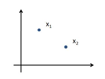
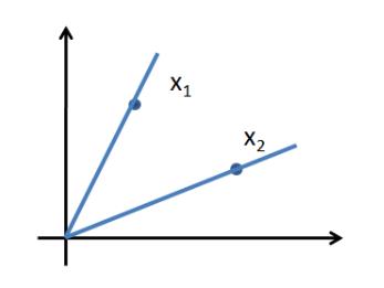
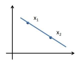
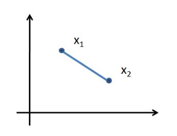
conical, and convex combinations, respectively. To get an intuitive feel of the above definitions, see Figure 1.
Definition 5. Given a convex set X ⊆ Rn, the affine dimension of X is the maximum number of affinely
independent points in X.

Figure 1: The subspace, cone set, affine set, and convex set of x , x (from left to right). Note that the
1
2
subspace is R2 and the cone set includes all points inside and on the two arrows.
1
.2 Polyhedra, Polytopes, and Cones
Definition 6 (Hyperplane, Halfspace). A hyperplane in Rn is the set of all points x ∈ Rn that satisfy
for some
a · x = b for some a ∈ R
n and ∈ R. A halfspace is the set of all points such that
b
x
a x
·
≤
b
a ∈ Rn and ∈ R.
b
Definition 7 (Polyhedron). A Polyhedron in Rn is the intersection of finitely many halfspaces. It can be
equivalently defined to be the set {x | Ax ≤ b} for a matrix A ∈ Rm×n and a vector b ∈ Rm×1.
Definition 8 (Polyhedral cone). A polyhedral cone is Rn the intersection of finitely many halfspaces that
contain the origin, i.e. {x | Ax ≤ 0} for a matrix A ∈ Rm×n.
Definition 9 (Polyotpe). A polytope is a bounded polyhedron.
Note that a polyhedron is a convex and closed set. It would be illuminating to classify a polyhedron into
the following four categories depending on how it looks.
1
2
3
4
. Empty set (when the system Ax ≤ b is infeasible.)
. Polytope (when the polyhedron is bounded.)
. Cone
. (Combination of) Cone and Polytope
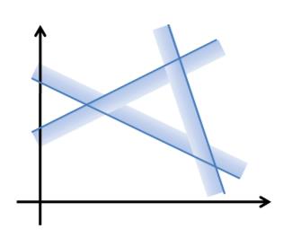
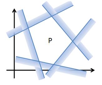
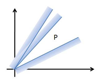
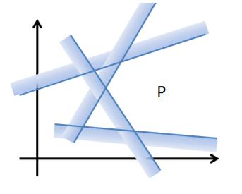
Figure 2: Examples of polyhedrons, left to right: Empty, Polytope, Cone, Combination of cone and polytope.
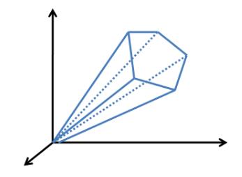
What “combination of cone and polytope” means will become clear soon in Theorem 12. For the
examples, the reader is referred to Figure 2. In 2-D, a cone can have only two “extreme rays,” while in 3-D
there is no bound on the number of extreme rays it can have.
For the most of part, we will be largely concerned with polytopes, but we need to have a better under-
standing of polyhedra first. Although it is geometrically “obvious” that a polytope is the convex hull of its
“
vertices,” the proof is quite non-trivial. We will state the following three theorems without proof.
Theorem 10. A bounded polyhedron is the convex hull of a finite set of points.
Theorem 11. A polyhedral cone is generated by a finite set of vectors. That is, for any A ∈ Rm×n, there
P
exists a finite set X such that {x =
Theorem 12. A polyhedron {x | Ax ≤ b} can be written as the Minkowski sum of a polytope Q and a cone
λ x | x ∈ X, λ ≥ 0} = {x | Ax ≤ 0}.
i
i
i
i
i
C, i.e. P = Q + C = {x + y | x ∈ Q, y ∈ C}.
One can (geometrically) obtain the Minkowski sum of a polytope Q and a cone C by sweeping the
origin of the cone C over the polytope Q. If the polyhedron P is pointed (has at least one “vertex”), the
decomposition is, in fact, modulo scaling factor unique. Further the cone C above is {x | Ax ≤ 0},
or equivalently the set of unbounded directions in P. The cone C is called the characteristic cone or the
recession cone of P.
Many facts about polyhedra and linear programming rely on (in addition to convexity) variants of Farkas’
lemma that characterizes when a system of linear inequalities do not have solution. The simplest proof for
one variant is via Fourier-Motzkin elimination that is independently interesting and related to the standard
Gauss-Jordan elimination for solving system of linear equations.
1
.2.1 Fourier-Motzkin Elimination
Let P = {x|Ax ≤ b} ⊆ Rn be a polyhedron. For k in [n],
we let Pk = {(x , .., x , x , ..., x ) | (x , x , ..., x ) ∈ P} be the projection of P along the x -axis.
1
k−1 k+1
n
1
2
n
k
Theorem 13. Pk is a polyhedron.
Proof. We derive a set of inequalities that describe Pk. We do this by considering the inequalities in Ax ≤ b
and eliminating the variables x as follows. Partition the inequalities in Ax ≤ b into three sets:
k
S+ = {i ∈ [m] | aik > 0}, S− = {i ∈ [m] | aik < 0},
and
S0 = {i ∈ [m] | aik = 0}.
Define a new set of inequalities consisting of S0 and one new inequality for each pair (i, `) in S+ × S−:
Xn
Xn
a (
ik
a x ) − a (
a x ) ≤ a b − a b .
`j
j
`k
ij
j
ik `
`k i
j=1
j=1
Note that the combined inequality does not have x . We now have a total of |S0| + |S+||S−| new
k
inequalities. Let P0 = {x0 ∈ Rn−1 | A0x0 ≤ b0} where A0x0 ≤ b0 is the new system of inequalities in
variables x , x , ..., x , x , ..., x . We prove the theorem by showing that Pk = P0.
1
2
k−1 k+1
n
We first show the easier direction: Pk ⊆ P0. Consider any point z ∈ Pk. By definition of Pk, there
exists x ∈ P such that Ax ≤ b and x’s projection along x -axis is z. It is easy to see that z satisfies the new
k
system since the new one was obtained in a way oblivious to x , the real value of x’s k coordinate.
k
th
We now show that P0 ⊆ Pk. Without loss of generality, assume k = 1. Consider any x0 = (x , x , ..., x ) ∈
2
3
n
0
. We want to show that there exists
R such that
, where
x = (x , x , ..., x )
. For simple
P
x ∈
Ax ≤ b
P
1
1
2
n
notation, define C = b −
n
j=2
a x for i ∈ [m]. Note that Ax ≤ b can be rewritten as
i
i
ij
j
a x ≤ C , ∀i ∈ [m].
(1)
i1
1
i
Observe that x satisfies all inequalities consisting of S0, since the new system as well includes those
constraints. Thus we can refine our goal to show
x1 s.t.
a x ≤ C , ∀i ∈ S+ ∪ S .
−
∃
i1
1
i
C
Ci
⇔
max`
∈S− a`1
`
≤ x ≤ min
i∈S+ ai1
.
1
It is easy to observe that this is equivalent to
C`
Ci
ai1
+
−
−
≤
, ∀(i, `) ∈ S × S
a`
1
⇔
⇔
0 ≤ a C − a C , ∀(i, `) ∈ S+ × S
i1
`
`1
i
A0x ≤ b0
0
And we know that A0x0 ≤ b0 since x0 ∈ P0, completing the proof.
From Fourier-Motzkin elimination we get an easy proof of one variant of Farkas’ lemma.
Theorem 14 (Theorem of Alternatives). Let A ∈ Rm×n and b ∈ Rm. For the system Ax ≤ b, exactly one
of the following two alternatives hold:
•
•
The system is feasible.
There exists y ∈ Rm such that y ≥ 0, yA = 0 and yb < 0.
What the theorem says is that if the system of inequalities Ax ≤ b is infeasible then there is a proof
(certificate) of this which can be obtained by taking non-linear combination of the inequalities (given by
y ≥ 0) to derive a contradiction of the following form: 0 = yA ≤ yb < 0.
Proof of [Theorem 14] Suppose that there exists a vector y0 ≥ 0 s.t. y0A = 0 and y0 · b < 0 and a vector x0
such that Ax0 ≤ b. Then it easily follows that 0 ≤ y0Ax0 ≤ y0b, since y0 ≥ 0, which is a contradiction to the
fact that y0b < 0.
Conversely, suppose Ax ≤ b is infeasible. Let P = {x | Ax ≤ b}. We eliminate variables x , x , ..., x
1
2
n
is
(we can choose any arbitrary order) to obtain polyhedra P = Q , Q , Q , ..., Q , Q . Note that Q
0
1
2
n−1
n
i+1
non-empty iff Qi is, and that Qn−1 has only one variable and Q has none. Note by the Fourier-Motzkin
n
elimination procedure the inequalities describing Q are non-negative combination of the inequalities of P;
i
this can be formally shown via induction. Thus, Qn is empty iff we have derived an inequality of the form
0
≤ C for some C < 0 at some point in the process. That inequality gives the desired y ≥ 0.
2
Two variant of Farkas’ lemma that are useful can be derived from the theorem of alternatives.
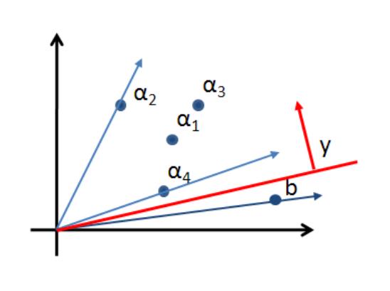
Theorem 15. Ax = b, x ≥ 0 has no solution iff ∃y ∈ Rm s.t. AT y ≥ 0 and bT y < 0.


The above theorem has a nice geometric interpretation. Let α , α , ..., α be the columns of A viewed as
1
2
n
vectors in Rm. Then Ax = b, x ≥ 0 has a solution if and only if b is in the cone generated by α , α , ..., α ;
1
2
n
here the combination is given by x ≥ 0. So b is either in the Cone(α , α , ..., α ) or there is a hyperplane
1
2
n
separating b from α , α , ..., α .
1
2
n
In fact the theorem can be strengthened to show that the hyperplane can be chosen to be one that spans
t − 1 linearly independent vectors in α , α , ..., α , where t = rank(α , α , ..., α , b).
1
2
n
1
2
n
Proof of [Theorem 15] We can rewrites Ax = b, x ≥ 0 as
A
b
−
A
x ≤ −b
−
I
0
Hence by the Theorem of Alternatives, Ax = b, x ≥ 0 is not feasible if and only if there exists a row vector
ꢂ
ꢃ
0
y = u v w
, where
are row vectors in Rm and is a row vector in Rn such that
u, v
w
u, v, w ≥ 0
uA − vA − w = 0
ub − vb < 0
Let y = u−v. Note that y ∈ Rm is now not necessarily positive. From the second and third inequalities,
we can easily obtain AT y ≥ 0 and bT y < 0.
2
Another variant of Farkas’ lemma is as follows and the proof is left as an exercise.
Theorem 16. Ax ≤ b, x ≥ 0 has a solution iff yb ≥ 0 for each row vector y ≥ 0 with yA ≥ 0.
Another interesting and useful theorem is Carathe´odory’s Theorem
Theorem 17 (Carathe´odory). Let x ∈ Convexhull(X) for a finite set X of points in Rn. Then x ∈
Convexhull(X0) for some X0 ⊆ X such that vectors in X0 are affinely independent. In particular,
0
.
|
X | ≤ n + 1
A conic variant of Carathe´odory’s Theorem is as follows.
Theorem 18. Let x ∈ Cone(X) where X = {x , x , ..., x }, x ∈ Rn. Then x ∈ Cone(X0) for some
1
2
m
i
0
where vectors in 0 are linearly independent. In particular,
0
.
X ⊆ X
X
|X | ≤ n
P
Proof. Since x ∈ Cone(X), x =
λ x for some λ ≥ 0. Choose a combination with mininum support,
i
i
i
i
i.e. the smallest number of non-zero λ values. Let X0 = {λ x | λ > 0} and I = {i | λ > 0}. If vectors
i
i
i
i
P
i
in X0 are linearly independent, we are done. Otherwise, ∃α , i ∈ I s.t.
α λ x = 0. By scaling we
i
∈
i
i
i
i
I
can assume that ∀i ∈ I, α ≤ 1, and ∃j ∈ I s.t. α = 1. Then,
i
j
X
X
X
X
X
0
0
i
x =
λ x =
i i
λ x −
α λ x =
i
λ (1 − α )x =
λ x (λ ≥ 0).
i
i
i
i
i
i
i
i
i
i∈I
i∈I
i∈I
i∈I
i∈I\{j}
This contradicts the fact that we chose the conical combination for x with the least support.
One can derive the affine version of Carathe´odory’s Theorem from the conical version, and the proof is
left as an exercise.
1
.3 Linear Programming
Linear programming is an optimization problem of the following form.
max c · x (Primal-LP)
Ax ≤ b
The above is one of the standard forms. In other words, we wish to maximize a linear objective function
over a polyhedron. Given an L P, there are three possibilities:
1
2
3
. The polyhedron is infeasible.
. The objective function can be made arbitrarily large in which case we can say it is unbounded.
. There is a finite optimum value in which case we say it is bounded.
Each linear program has its associated “dual” linear program. The LP we refer to by “dual” depends
on the “starting” L P, which is called as the primal LP; in fact the dual of dual LP is exactly the same as the
primal LP. Let us say that the following LP is the primal LP here.
max c · x
Ax ≤ b
We can “derive” the dual by thinking about how we can obtain an upper bound on the optimal value
for the primal L P. Given the system Ax ≤ b, any inequality obtained by non-negative combination of the
inequalities in Ax ≤ b is a valid inequality for the system. We can represent a non-negative combination by
a m × 1 row vector y ≥ 0.
Thus yAx ≤ yb is a valid inequality for y ≥ 0. Take any vector y0 ≥ 0 s.t. y0A = c. Then such a vector
gives us an upperbound on the LP value since y0Ax = cx ≤ y0b is a valid inequality. Therefore one can
obtain an upperbound by minimizing over all y0 ≥ 0 s.t. y0A = c. Therefore the objective function of the
primal LP is upperbounded by the optimum value of
min yb (Dual-LP)
yA = c
y ≥ 0
The above derivation of the Dual LP immediately implies the Weak Duality Theorem.

Theorem 19 (Weak Duality). If x0 and y0 are feasible solutions to Primal-LP and Dual-LP then cx0 ≤ y0b.
Corollary 20. If the primal-LP is unbounded then the Dual-LP is infeasible.
Exercise: Prove that the dual of the Dual-LP is the Primal-LP.
The main result in the theory of linear programming is the following Strong Duality Theorem which is
essentially a min-max result.
Theorem 21 (Strong Duality). If Primal-LP and Dual-LP have feasible solutions, then there exist feasible
solutions x∗ and y∗ such that cx∗ = y∗b.
Proof. Note that by weak duality we have that cx0 ≤ y0b for any feasible pair of x0 and y0. Thus to show
the existence of x∗ and y∗ it suffices to show that the system of inequalities below has a feasible solution
whenever the two LPs are feasible.
cx ≥ yb
Ax ≤ b
yA = c
y ≥ 0
We rewrite this as
Ax ≤ b
yA ≤ c
−
yA ≤ −c
−
y ≤ 0
−
cx + yb ≤ 0
and apply the Theorem of Alternatives. Note that we have inequalities in n + m variables corresponding to
ꢄ
ꢅ
x
yT
the x and y variables. By expressing those variables as a vector z =
, we have
A
0
0
0
AT
−A
−I
bT
b
cT
ꢄ
ꢅ
x
y
T
T
≤ −c
0
0
0
−
c
ꢂ
ꢃ
If the above system does not have a solution then there exists a vector s t t0 u v ≥ 0, where s
is a m × 1 row vector, t, t0 are n × 1 row vectors, u is a m × 1 row vector and v is a scalar such that
sA − v · c = 0
T
0
T
tA − t A − u + v · b = 0
sb + t · c − t · c0 < 0
We replace t−t0 by w and note that now w is not necessarily positive. Hence we obtain that if the strong
duality does not hold then there exist vectors s, u ∈ Rm, w ∈ Rn, v ∈ R such that
s, u, v ≥ 0
sA − v · c = 0
T
wA − u + v · b = 0
sb + wcT < 0
We consider two cases.
Case 1: v = 0. (note that v is a scalar.)
In this case, the above system simplifies to
s ≥ 0
sA = 0
wAT = 0
sb + wcT < 0
Since we have y∗A = c and sA = 0, y∗ + αs is a feasible solution for the dual for any scalar α ≥ 0.
Similarly knowing that Ax∗ ≤ b and AwT = 0 (from wAT = 0), it follows that x∗ − αwT is feasible for
the primal for any scalar α ≥ 0. Applying the Weak Duality Theorem, we have that ∀α ≥ 0,
∗
T
∗
c(x − αw ) ≤
(y + αs) · b
∗
∗
T
⇒
cx − y b
≤ α(s · b + c · w )
However, the LHS is fixed while the RHS can be made arbitrarily small because s · b + c · wT < 0 and α
can be chosen arbitrarily large.
Case 2: v > 0.
Let s0 = 1 (s), w0 = 1 (w), and u0 = 1 (u). Then, we have
v
v
v
s0, u0 ≥ 0
s A = c
0
0
T
0
0 T
0
[Since
u0 ≥ 0
.]
w A − u = −b ⇒ −A(w ) = b − u ≤ b
< 0
0
s b + w c
0 T
From the inequalities above, we observe that s0 is dual feasible and −w0 is primal feasible. Thus by the
Weak Duality, we have −w0 · cT ≤ s0b, contradicting that s0b + w · cT < 0.
Finally, we make a remark on where the contradiction really comes from for each case. For the first case
where v = 0, note that the inequality −cx + yb ≤ 0, which forces the optimal values for the primal and
the dual meet each other, was never used. In other words, we got a contradiction because there do not exist
feasible solutions satisfying both the primal and the dual. On the other hand, for the second case v > 0,
we had feasible solutions for both LPs, but obtained a contradiction essentially from the assumption that the
two optimal values are different.
Complementary Slackness is a very useful consequence of Strong Duality.
Theorem 22 (Complementary Slackness). Let x∗, y∗ be feasible solutions to the primal and dual LPs. Then
x∗, y∗ are optimal solutions if and only if ∀i ∈ [m]
, either
∗
or
y = 0 a x = b
∗
.
i
i
i


Proof. Let α , α , ...α be the row vectors of A. Suppose that the given condition is satisfied. Then we
1
P2
m
P
have y∗Ax∗ = m y∗(α x∗) = m y∗b = y∗b. Also we know that cx∗ = y∗Ax∗ since y∗ is a feasible
i
i
i
i=1
i
i=1
solution for the dual. Thus we have cx∗ = y∗b, and by the Weak Duality, we conclude that x∗, y∗ are
optimal.
Conversely, suppose that x∗ and y∗ both are optimal. Then by the Strong Duality and because x∗, y∗
are feasible, we have that y∗b = cx∗ = y∗Ax∗ ≤ y∗b. Thus we obtain the equality y∗Ax∗ = y∗b, that is
P
P
m
i=1
∗
∗
m
i=1
∗ . This equality forces the desired condition, since
∗
∗
i
because
y (α x ) =
y b
α x ≤ b , y ≥ 0
i
i
i
i
i
i
∗
and ∗ are feasible solutions.
x
y
References
[
[
[
1] L. Schrijver. Theory of Linear and Integer Programming (Paperback). Wiley, Chapters 7, 8, 1998.
2] J. Lee. A First Course in Combinatorial Optimization. Cambridge University Press, 2004.
3] M. Goemans. Lecture notes on linear programming and polyhedral combinatorics. http://www-
math.mit.edu/ goemans/18433S09/polyhedral.pdf, 2009.

Massachusetts Institute of Technology
8.433: Combinatorial Optimization
Michel X. Goemans
Handout 6
February 20th, 2009
1
3
. Linear Programming and Polyhedral Combinatorics
Summary of what was seen in the introductory lectures on linear programming and
polyhedral combinatorics.
aD∈efiRnnitaionnd b3 .∈1RA. halfspace in Rn is a set of the form {x ∈ Rn : aT x ≤ b} for some vector
Definition 3.2 A polyhedron is the intersection of finitely many halfspaces: P = {x ∈ Rn :
Ax ≤ b}.
Definition 3.3 A polytope is a bounded polyhedron.
Definition 3.4 If P is a polyhedron in Rn, the projection P ⊆ Rn of P is defined as
−
1
k
{
y = (x , x , · · · , x , x , · · · , x ) : x ∈ P for some x }.
k−1
1
2
k+1
n
k
This is a special case of a projection onto a linear space (here, we consider only coordinate
projection). By repeatedly projecting, we can eliminate any subset of coordinates.
We claim that Pk is also a polyhedron and this can be proved by giving an explicit
description of Pk in terms of linear inequalities. For this purpose, one uses Fourier-Motzkin
elimination. Let P = {x : Ax ≤ b} and let
•
•
•
S = {i : a > 0},
+
ik
S = {i : a < 0},
−
ik
S = {i : a = 0}.
0
ik
Clearly, any element in P must satisfy the inequality aT x ≤ b for all i ∈ S (these inequal-
k
ities do not involve x ). Similarly, we can take a linear combination of an inequality in S
i
i
0
k
and one in S to eliminate the coefficient of x . This shows that the inequalities:
+
−
k
!
!
X
X
aik
a x − alk
a xj ≤ a b − a b
(1)
lj
j
ij
ik
l
lk
i
j
j
for i ∈ S and l ∈ S are satisfied by all elements of Pk. Conversely, for any vector
+
−
(x , x , · · · , x , x , · · · , x ) satisfying (1) for all i ∈ S and l ∈ S and also
1
2
k−1
k+1
n
+
−
T
i
a x ≤ b for all i ∈ S
(2)
i
0
we can find a value of xk such that the resulting x belongs to P (by looking at the bounds on
xk that each constraint imposes, and showing that the largest lower bound is smaller than
the smallest upper bound). This shows that Pk is described by (1) and (2), and therefore is
a polyhedron.

3
. Linear Programming and Polyhedral Combinatorics
February 20th, 2009
2
Definition 3.5 Given points a(1), a(2), · · · , a(k) ∈ Rn,
P
•
•
•
•
a linear combination is
an affine combination is
a conical combination is
a convex combination is
λ a(i) where λ ∈ R for all i,
i
i
i
P
P
λ a(i) where λ ∈ R and
λi = 1,
i
i
i
i
P
λ a(i) where λ ≥ 0 for all i,
i
i
i
P
P
λ a(i) where λ ≥ 0 for all i and
λi = 1.
i
i
i
i
The set of all linear combinations of elements of S is called the linear hull of S and
denoted by lin(S). Similarly, by replacing linear by affine, conical or convex, we define the
affine hull, aff(S), the conic hull, cone(S) and the convex hull, conv(S). We can give an
equivalent definition of a polytope.
Definition 3.6 A polytope is the convex hull of a finite set of points.
The fact that Definition 3.6 implies Definition 3.3 can be shown by using Fourier-Motzkin
elimination repeatedly on
X
x −
λka(k) = 0
k
X
λk = 1
k
λk ≥ 0
to eliminate all variables λk and keep only the variables x. The converse will be discussed
later in these notes.
3
.1 Solvability of System of Inequalities
In linear algebra, we saw that, for A ∈ Rm×n, b Rm, Ax = b has no solution x
∈
∈ Rn
if
and only if there exists a y ∈ Rm with AT y = 0 and bT y = 0 (in 18.06 notation/terminology,
this is equivalent to saying that the column space C(A) is orthogonal to the left null space
N(AT )).
One can state a similar Theorem of the Alternatives for systems of linear inequalities.
Theorem 3.1 (Theorem of the Alternatives) Ax ≤ b has no solution x ∈ Rn if and
only if there exists y ∈ Rm such that y ≥ 0, AT y = 0 and bT y < 0.
One can easily show that both systems indeed cannot have a solution since otherwise
0
> bT y = yT b ≥ yT Ax = 0T x = 0. For the other direction, one takes the insolvable system
Ax ≤ b and use Fourier-Motzkin elimination repeatedly to eliminate all variables and thus
obtain an inequality like 0T x ≤ c where c < 0. In the process one has derived a vector y
with the desired properties (as Fourier-Motzkin only performs nonnegative combinations of
linear inequalities).
Another version of the above theorem is Farkas’ lemma:
3
. Linear Programming and Polyhedral Combinatorics
February 20th, 2009
3
bLTeym<m0a. 3.2 Ax = b, x ≥ 0 has no solution if and only if there exists y with AT y ≥ 0 and
Exercise 3-1. Prove Farkas’ lemma from the Theorem of the Alternatives.
3
.2 Linear Programming Basics
A linear program (LP) is the problem of minimizing or maximizing a linear function over a
polyhedron:
Max cT x
subject to:
(P)
Ax ≤ b,
where A ∈ Rm×n, b
∈ Rm
, c
∈ Rn
and the variables x are in Rn. Any x satisfying Ax
≤
b
is said to be feasible. If no x satisfies Ax ≤ b, we say that the linear program is infeasible,
and its optimum value is −∞ (as we are maximizing over an empty set). If the objective
function value of the linear program can be made arbitrarily large, we say that the linear
program is unbounded and its optimum value is +∞; otherwise it is bounded. If it is neither
infeasible, not unbounded, then its optimum value is finite.
Other equivalent forms involve equalities as well, or nonnegative constraints x ≥ 0.
One version that is often considered when discussing algorithms for linear programming
(especially the simplex algorithm) is min{cT x : Ax = b, x ≥ 0}.
Another linear program, dual to (P), plays a crucial role:
Min bT y
subject to:
(D)
AT y = c
y ≥ 0.
(D) is the dual and (P) is the primal. The terminology for the dual is similar. If (D)
has no feasible solution, it is said to be infeasible and its optimum value is +∞ (as we are
minimizing over an empty set). If (D) is unbounded (i.e. its value can be made arbitrarily
negative) then its optimum value is −∞.
The primal and dual spaces should not be confused. If A is m×n then we have n primal
variables and m dual variables.
Weak duality is clear: For any feasible solutions x and y to (P) and (D), we have that
cT x ≤ bT y. Indeed, cT x = yT Ax ≤ bT y. The dual was precisely built to get an upper bound
on the value of any primal solution. For example, to get the inequality yT Ax ≤ bT y, we need
that y ≥ 0 since we know that Ax ≤ b. In particular, weak duality implies that if the primal
is unbounded then the dual must be infeasible.
Strong duality is the most important result in linear programming; it says that we can
prove the optimality of a primal solution x by exhibiting an optimum dual solution y.
3
. Linear Programming and Polyhedral Combinatorics
February 20th, 2009
4
Theorem 3.3 (Strong Duality) Assume that (P) and (D) are feasible, and let z∗ be the
∗
optimum value of the primal and w the optimum value of the dual. Then z = w .
∗
∗
The proof of strong duality is obtained by writing a big system of inequalities in x and y
which says that (i) x is primal feasible, (ii) y is dual feasible and (iii) cT x ≥ bT y. Then use
the Theorem of the Alternatives to show that the infeasibility of this system of inequalities
would contradict the feasibility of either (P) or (D).
∗
Let x be a feasible solution to the primal, and y be a feasible solution to the
dual. The proof is by contradiction. Because of weak duality, this means that there are no
∗
Proof:
solution x ∈ Rn and y ∈ Rm such that
Ax
≤ b
AT y = c
Iy
cT x +bT y ≤ 0
≤ 0
−
By a variant of the Theorem of the Alternatives or Farkas’ lemma (for the case when we
have a combination of inequalities and equalities), we derive that there must exist s ∈ Rm,
t ∈ Rn, u ∈ Rm, v ∈ R such that:
s ≥ 0
u ≥ 0
v ≥ 0
T
A s − vc = 0
At − u + vb = 0
b s + c t < 0.
T
T
We distinguish two cases.
Case 1: v = 0. Then s satisfies s ≥ 0 and AT s = 0. This means that, for any α ≥ 0,
y + αs is feasible for the dual. Similarly, At = u 0 and therefore, for any α 0, we have
≥
∗
≥
that x∗ αt is primal feasible. By weak duality, this means that, for any α 0, we have
−
≥
T
∗
T
∗
c (x − αt) ≤ b (y + αs)
or
T
∗
T
∗
T
T
c x − b y ≤ α(b s + c t).
The right-hand-side tend to −∞ as α tends to ∞, and this is a contradiction as the left-
hand-side is fixed.
3
. Linear Programming and Polyhedral Combinatorics
February 20th, 2009
5
Case 2: v > 0. By dividing throughout by v (and renaming all the variables), we get that
there exists s ≥ 0, u ≥ 0 with
AT s = c
At − u = −b
b s + c t < 0.
T
T
This means that s is dual feasible and −t is primal feasible, and therefore by weak duality
cT (−t) ≤ bT s contradicting bT s + cT t < 0.
4
Exercise 3-2. Show that the dual of the dual is the primal.
Exercise 3-3. Show that we only need either the primal or the dual to be feasible for
strong duality to hold. More precisely, if the primal is feasible but the dual is infeasible,
∗
prove that the primal will be unbounded, implying that z = w = + .
∗
∞
Looking at cT x = yT Ax ≤ bT y, we observe that to get equality between cT x and bT y, we
need complementary slackness:
Theorem 3.4 (Complementary Slackness) If x is feasible in (P) and y is feasible in
(D) then x is optimum in (P) and y is optimum in (D) if and only if for all i either y = 0
P
Linear programs can be solved using the simplex method; this is not going to be explained
i
or
a x = b (or both).
ij
j
i
j
in these notes. No variant of the simplex method is known to provably run in polynomial
time, but there are other polynomial-time algorithms for linear programming, namely the
ellipsoid algorithm and the class of interior-point algorithms.
3
.3 Faces of Polyhedra
P
Definition 3.7 {a(i) ∈ Rn : i ∈ K} are linearly independent if
λ = 0 for all i ∈ K.
λia(i) = 0 implies that
i
i
P
P
Definition 3.8 {a(i) ∈ Rn : i ∈ K} are affinely independent if
λia(i) = 0 and
λi = 0
i
i
together imply that λ = 0 for all i ∈ K.
i
Observe that {a(i) ∈ Rn : i ∈ K} are affinely independent if and only if
ꢀ
ꢁ
ꢂ
ꢃ
a(i)
1
∈
Rn+1 : i ∈ K
are linearly independent.
Definition 3.9 The dimension, dim(P), of a polyhedron P is the maximum number of
affinely independent points in P minus 1.
3
. Linear Programming and Polyhedral Combinatorics
February 20th, 2009
6
The dimension can be -1 (if P is empty), 0 (when P consists of a single point), 1 (when
P is a line segment), and up to n when P affinely spans Rn. In the latter case, we say that
P is full-dimensional. The dimension of a cube in R3 is 3, and so is the dimension of R3
itself (which is a trivial polyhedron).
Definition 3.10 αT x ≤ β is a valid inequality for P if αT x ≤ β for all x ∈ P.
Observe that for an inequality to be valid for conv(S) we only need to make sure that
it is satisfied by all elements of S, as this will imply that the inequality is also satisfied by
points in conv(S) \ S. This observation will be important when dealing with convex hulls of
combinatorial objects such as matchings or spanning trees.
Definition 3.11 A face of a polyhedron P is {x ∈ P : αT x = β} where αT x ≤ β is some
valid inequality of P.
By definition, all faces are polyhedra. The empty face (of dimension -1) is trivial, and so
is the entire polyhedron P (which corresponds to the valid inequality 0T x ≤ 0). Non-trivial
are those whose dimension is between 0 and dim(P) − 1. Faces of dimension 0 are called
extreme points or vertices, faces of dimension 1 are called edges, and faces of dimension
dim(P) − 1 are called facets. Sometimes, one uses ridges for faces of dimension dim(P) − 2.
Exercise 3-4. List all 28 faces of the cube P = {x ∈ R3 : 0 ≤ xi ≤ 1 for i = 1, 2, 3}.
Although there are infinitely many valid inequalities, there are only finitely many faces.
Theorem 3.5 Let A ∈ Rm . Then any non-empty face of P = x
×
n
{
∈ Rn
: Ax
≤ }
b
corresponds to the set of solutions to
X
a x = b for all i ∈ I
ij
j
i
j
X
a x ≤ b for all i ∈/ I,
ij
j
i
j
for some set I ⊆ {1, · · · , m}. Therefore, the number of non-empty faces of P is at most 2m.
Proof:
Consider any valid inequality αT x ≤ β. Suppose the corresponding face F is
non-empty. Thus F are all optimum solutions to
Max αT x
subject to:
(P)
Ax ≤ b.
3
. Linear Programming and Polyhedral Combinatorics
February 20th, 2009
7
Choose an optimum solution y∗ to the dual LP. By complementary slackness, the face F is
defined by those elements x of P such that aT x = b for i ∈ I = {i : y > 0 . Thus F is
∗
i
}
i
i
defined by
X
a x = b for all i ∈ I
ij
j
i
j
X
a x ≤ b for all i ∈/ I.
ij
j
i
j
As there are 2m possibilities for F, there are at most 2m non-empty faces.
The number of faces given in Theorem 3.5 is tight for polyhedra (see exercise below), but
4
can be considerably improved for polytopes in the so-called upper bound theorem.
Exercise 3-5. Let P = {x ∈ Rn : x ≥ 0 for i = 1, · · · , n}. Show that P has 2n + 1 faces.
i
How many faces of dimension k does P have?
For extreme points (faces of dimension 0), the characterization is even stronger (we do
not need the inequalities):
Theorem 3.6 Let x be an extreme point for P = x : Ax ≤ b}. Then there exists I such
∗
{
that x∗ is the unique solution to
X
a x = b for all i ∈ I.
ij
j
i
j
P
∗
Given an extreme point x , define I by I = i :
{
a x = b . This means that
}
∗
Proof:
for i ∈/ I, we have
P
j
ij
j
i
∗
a x < b .
ij
From Theorem 3.5, we know that x is uniquely defined by
j
i
j
∗
X
a x = b for all i ∈ I
(3)
(4)
ij
j
i
j
X
a x ≤ b for all i ∈/ I.
ij
j
i
j
Now suppose there exists another solution xˆ when we consider only the equalities for i ∈ I.
P
Then because of
sufficiently small. A contradiction (as the face was supposed to contain a single point).
a x < b , we get that (1 ꢀ)x + ꢀxˆ also satisfies (3) and (4) for ꢀ
−
∗
∗
ij
j
i
j
4
If P is given as {x : Ax = b, x ≥ 0} (as is often the case), the theorem still applies (as
we still have a system of inequalities). In this case, the theorem says that every extreme
point x∗ can be obtained by setting some of the variables to 0, and solving for the unique
solution to the resulting system of equalities. Without loss of generality, we can remove from
Ax = b equalities that are redundant; this means that we can assume that A has full row
rank (rank(A) = m for A ∈ Rm×n). Letting N denote the indices of the non-basic variables
that we set of 0 and B denote the remaining indices (of the so-called basic variables), we
3
. Linear Programming and Polyhedral Combinatorics
February 20th, 2009
8
∗
∗
∗
N
can partition x into x and x (corresponding to these two sets of variables) and rewrite
B
Ax = b as A x +A x = b, where A and A are the restrictions of A to the indices in B
B
and N respectively. The theorem says that x is the unique solution to A x + A x = 0
B
N
N
B
N
∗
∗
B
B
B
N
and x = 0, which means x = 0 and A x = b. This latter system must have a unique
N
∗
N
N
B
solution, which means that A must have full column rank (rank(A ) = |B|). As A itself
B
B
has rank m, we have that |B| ≤ m and we can augment B to include indices of N such that
the resulting B satisfies (i) |B| = m and (ii) A is a m×m invertible matrix (and thus there
B
is still a unique solution to A x = b). In linear programming terminology, a basic feasible
B
B
solution or bfs of {x : Ax = b, x ≥ 0} is obtained by choosing a set |B| = m of indices with
−
1
A invertible and letting x = A b and x = 0 where N are the indices not in B. All
B
B
B
N
extreme points are bfs and vice versa (although two different bases B may lead to the same
extreme point, as there might be many ways of extending A into a m×m invertible matrix
B
in the discussion above).
One consequence of Theorem 3.5 is:
Corollary 3.7 The maximal (inclusion-wise) non-trivial faces of a non-empty polyhedron
P are the facets.
For the vertices, one needs one additional condition:
Corollary 3.8 If rank(A) = n (full column rank) then the minimal (inclusion-wise) non-
trivial faces of a non-empty polyhedron P = {x ∈ Rn : Ax ≤ b} are the vertices.
Exercise 3-7 shows that the rank condition is necessary.
This means that, if a linear program max{cT x : x ∈ P} with P = {x : Ax ≤ b} is
feasible, bounded and rank(A) = n, then there exists an optimal solution which is a vertex
of P (indeed, the set of all optimal solutions define a face — the optimal face — and if this
face is not itself a vertex of P, it must contain vertices of P).
We now prove Corollary 3.8.
Proof:
have a set I such that
Let F be a minimal (inclusion-wise) non-trivial face of F. This means that we
F = {x : aT x = b i ∈ I
i
i
aT x ≤ b j ∈/ I}
j
j
and adding any element to I makes this set empty. Consider two cases. Either P = {x ∈
Rn : aT x = b for i ∈ I} or not. In the first case, it means that for every j ∈/ I we have
i
i
a ∈ lin({a : i ∈ I}) and therefore since rank(A) = n we have that the system aT x = b for
j
i
i
i
i ∈ I has a unique solution and thus F is a vertex.
On the other hand, if P = {x ∈ Rn : aT x = b for i ∈ I} then let j ∈/ I such that there
i
i
exists x˜ with
aTi x˜ = bi i ∈ I
aT x˜ > b .
j
j
Since F is not trivial, there exists xˆ ∈ F, and in particular, xˆ satisfies
aTi xˆ = bi i ∈ I
aT xˆ ≤ b .
j
j
3
. Linear Programming and Polyhedral Combinatorics
February 20th, 2009
9
0
Thus for a suitable convex combination x of xˆ and x˜, we have a x = b for i
T
0
∈
j ,
∪ { }
I
i
i
contrdicting the maximality of I.
We now go back to the equivalence between Definitions 3.3 and 3.6 and claim that we
can show that Definition 3.3 implies Definition 3.6.
4
Theorem 3.9 If P = {x : Ax ≤ b} is bounded then P = conv(X) where X is the set of
extreme points of P.
This is a nice exercise using the Theorem of the Alternatives.
Since X ⊆ P, we have conv(X) ⊆ P. Assume, by contradiction, that we do not
Proof:
have equality. Then there must exist x˜ ∈ P \ conv(X). The fact that x˜ ∈/ conv(X) means
that there is no solution to:
P
λvv = x˜
λv = 1
λ ≥ 0
P
v∈X
v∈X
v ∈ X.
v
By the Theorem of the alternatives, this implies that ∃c ∈ Rn, t ∈ R:
ꢀ
P
n
j=1
t +
t +
c v ≥ 0 ∀v ∈ X
P
j
c x˜ < 0.
j
n
j
j
j=1
Since P is bounded, min{cT x : x ∈ P} is finite (say equal to z ), and the face induced by
∗
cT x ≥ z is non-empty but does not contain any vertex (as all vertices are dominated by x˜
∗
by the above inequalities). This is a contradiction with Corollary 3.8.
4
When describing a polyhedron P in terms of linear inequalities, the only inequalities that
are needed are the ones that define facets of P. This is stated in the next few theorems. We
say that an inequality in the system Ax ≤ b is redundant if the corresponding polyhedron is
unchanged by removing the inequality. For P = {x : Ax ≤ b}, we let I denote the indices
=
i such that aT x = b for all x ∈ P, and I the remaining ones (i.e. those for which there
i
i
<
exists x ∈ P with aT x < b ).
i
i
This theorem shows that facets are sufficient:
Theorem 3.10 If the face associated with aT x ≤ b for i ∈ I is not a facet then the
i
i
<
inequality is redundant.
And this one shows that facets are necessary:
Theorem 3.11 If F is a facet of P then there must exists i ∈ I such that the face induced
<
by aT x ≤ b is precisely F.
i
i
In a minimal description of P, we must have a set of linearly independent equalities
together with precisely one inequality for each facet of P.
3
. Linear Programming and Polyhedral Combinatorics
February 20th, 2009
10
Exercises
Exercise 3-6. Prove Corollary 3.7.
Exercise 3-7. Show that if rank(A) < n then P = {x ∈ Rn : Ax ≤ b} has no vertices.
Exercise 3-8. Suppose P = {x ∈ Rn : Ax ≤ b, Cx ≤ d}. Show that the set of vertices of
Q = {x ∈ Rn : Ax ≤ b, Cx = d} is a subset of the set of vertices of P.
(In particular, this means that if the vertices of P all belong to {0, 1}n, then so do the
vertices of Q.)
Exercise 3-9. Given two extreme points a and b of a polyhedron P, we say that they
are adjacent if the line segment between them forms an edge (i.e. a face of dimension 1) of
the polyhedron P. This can be rephrased by saying that a and b are adjacent on P if and
only if there exists a cost function c such that a and b are the only two extreme points of P
minimizing cT x over P.
Consider the polyhedron (polytope) P defined as the convex hull of all perfect matchings
in a (not necessarily bipartite) graph G. Give a necessary and sufficient condition for two
matchings M and M to be adjacent on this polyhedron (hint: think about M 4 M =
1
2
1
2
(M \ M ) ∪ (M \ M )) and prove that your condition is necessary and sufficient.)
1
2
2
1
Exercise 3-10. Show that two vertices u and v of a polyhedron P are adjacent if and
1
only there is a unique way to express their midpoint ( (u + v)) as a convex combination of
vertices of P.
2
3
.4 Polyhedral Combinatorics
In one sentence, polyhedral combinatorics deals with the study of polyhedra or polytopes as-
sociated with discrete sets arising from combinatorial optimization problems (such as match-
ings for example). If we have a discrete set X (say the incidence vectors of matchings in a
graph, or the set of incidence vectors of spanning trees of a graph, or the set of incidence
vectors of stable sets1 in a graph), we can consider conv(X) and attempt to describe it in
terms of linear inequalities. This is useful in order to apply the machinery of linear program-
ming. However, in some (most) cases, it is actually hard to describe the set of all inequalities
defining conv(X); this occurs whenever optimizing over X is hard and this statement can be
made precise in the setting of computational complexity. For matchings, or spanning trees, or
several other structures (for which the corresponding optimization problem is polynomially
solvable), we will be able to describe their convex hull in terms of linear inequalities.
Given a set X and a proposed system of inequalities P = {x : Ax ≤ b}, it is usually easy
to check whether conv(X) ⊆ P. Indeed, for this, we only need to check that every member
of X satisfies every inequality in the description of P. The reverse inclusion is more difficult.
1
A set S of vertices in a graph G = (V, E) is stable if there are no edges between any two vertices of S.


3
. Linear Programming and Polyhedral Combinatorics
February 20th, 2009
11
Here are 3 general techniques to prove that P ⊆ conv(X) (if it is true!) (once we know that
conv(X) ⊆ P).
1
. Algorithmically. This involves linear programming duality. This is what we did
in the notes about the assignment problem (minimum weight matchings in bipartite
graphs). In general, consider any cost function c and consider the combinatorial opti-
mization problem of maximizing cT x over x ∈ X. We know that:
T
T
max{c x : x ∈ X} = max{c x : x ∈ conv(X)}
T
≤
max{c x : Ax ≤ b}
T
T
=
min{b y : A y = c, y ≥ 0},
the last equality coming from strong duality. If we can exhibit a solution x ∈ X (say
a perfect matching in the assignment problem) and a dual feasible solution y (values
u , v in the assignment problem) such that cT x = bT y we will have shown that we
i
j
have equality throughout, and if this is true for any cost function, this implies that
P = conv(X).
This is usually the most involved approach but also the one that works most often.
2
. Focusing on extreme points. Show first that P = {x : Ax ≤ b} is bounded (thus a
polytope) and then study its extreme points. If we can show that every extreme point
of P is in X then we would be done since P = conv(ext(P)) ⊆ conv(X), where ext(P)
denotes the extreme points of P (see Theorem 3.9). The assumption that P is bounded
is needed to show that indeed P = conv(ext(P)) (not true if P is unbounded).
In the case of the convex hull of bipartite matchings, this can be done easily and this
leads to the notion of Totally Unimodular Matrices (TUM), see the next section.
3
. Focusing on the facets of conv(X). This leads usually to the shortest and cleanest
proofs. Suppose that our proposed P is of the form {x ∈ Rn : Ax ≤ b, Cx = d}. We
have already argued that conv(X) ⊆ P and we want to show that P ⊆ conv(X).
First we need to show that we are not missing any equality. This can be done for
example by showing that dim(conv(X)) = dim(P) (i.e. showing that if there are n−d
linearly independent rows in C we can find d + 1 affinely independent points in X).
Then we need to show that we are not missing a valid inequality that induces a facet
of conv(X). Consider any valid inequality αT x ≤ β for conv(X) with α = 0. We can
assume that α is any vector in Rn \ {0} and that β = max{αT x : x ∈ conv(X)}. The
face of conv(X) this inequality defines is F = conv({x ∈ X : αT x = β}). Assume that
this is a non-trivial face; this will happen precisely when α is not in the row space of
C. We need to make sure that if F is facet then we have in our description of P an
inequality representing it. What we will show is that if F is non-trivial then we can find
an inequality aT x ≤ b in our description of P such that F ⊆ {x : aT x = b }, or simply
i
i
i
i
3
. Linear Programming and Polyhedral Combinatorics
February 20th, 2009
12
that every optimum solution to max{αT x : x ∈ X} satisfies aT x = b . This means that
i
i
if F was a facet, by maximality, we have a representative of F in our description.
This is a very simple and powerful technique, and this is best illustrated on an example.
Example. Let X = {(σ(1), σ(2), · · · , σ(n)) : σ is a permutation of {1, 2, · · · , n}}. We
claim that
P
ꢄ
ꢅ
conv(X) = {x ∈ Rn :
n
i=1
xi =
xi ≥
n+1
2
P
ꢄ|
ꢅ
S|+1
S ⊂ {1, · · · , n}}.
i∈S
2
This is known as the permutahedron.
Here conv(X) is not full-dimensional; we only need to show that we are not missing
any facets and any equality in the description of conv(P). For the equalities, this
can be seen easily as it is easy to exhibit n affinely independent permutations in
X. For the facets, suppose that αT x ≤ β defines a non-trivial facet F of conv(X).
Consider maximizing αT x over all permutations x. Let S = arg min{α }; by our
i
assumption that F is non-trivial we have that S = {1, 2, · · · , n} (otherwise, we would
P
ꢄ
ꢅ
n
i=1
n+1
2
have the equality
x =
i
). Moreover, it is easy to see (by an exchange
argument) that any permutationσ whose incidence vector x maximizes αT x will need
to satisfy σ(i) ∈ {1, 2, · · · , |S|} for i ∈ S, in other words, it will satisfy the inequality
P
ꢄ
ꢅ
|
S|+1
x ≥
at equality. Hence, F is contained in the face corresponding to an
inequality in our description, and hence our description contains inequalities for all
facets. This is what we needed to prove. That’s it!
i∈S
i
2
Exercises
Exercise 3-11. Consider the set X = {(σ(1), σ(2), · · · , σ(n)) : σ is a permutation of
{
1, 2 · · · , n}}. Show that dim(conv(X)) = n − 1. (To show that dim(conv(X)) ≥ n − 1, ex-
hibit n affinely independent permutations σ (and prove that they are affinely independent).)
Exercise 3-12. A stable set S (sometimes, it is called also an independent set) in a graph
G = (V, E) is a set of vertices such that there are no edges between any two vertices in S.
If we let P denote the convex hull of all (incidence vectors of) stable sets of G = (V, E), it
is clear that x + x ≤ 1 for any edge (i, j) ∈ E is a valid inequality for P.
i
j
1
.Give a graph G for which P is not equal to
{
x ∈ R|V | : x + x ≤ 1 for all (i, j) ∈ E
i
j
x ≥ 0
.Show that if the graph G is bipartite then P equals
for all i ∈ V }
i
2
{
x ∈ R|V | : x + x ≤ 1 for all (i, j) ∈ E
i
j
x ≥ 0
for all i ∈ V }.
i
3
. Linear Programming and Polyhedral Combinatorics
February 20th, 2009
13
Exercise 3-13. Let e ∈ Rn (k = 0, . . . , n − 1) be a vector with the first k entries being
k
1
, and the following n − k entries being −1. Let S = {e , e , . . . , e , −e , −e , . . . , −e },
0
1
n−1
0
1
n−1
i.e. S consists of all vectors consisting of +1 followed by −1 or vice versa. In this problem
set, you will study conv(S).
P
n
i=1
1
.Consider any vector a ∈ {−1, 0, 1}n such that (i)
ai = 1 and (ii) for all j =
P
j
i=1
1
, . . . , n−1, we have 0 ≤
a ≤ 1. (For example, for n = 5, the vector (1, 0, −1, 1, 0)
i
P
P
n
i=1
n
i=1
satisfies these conditions.) Show that
inequalities for conv(S).
a x ≤ 1 and
a x ≥ −1 are valid
i
i
i
i
2
3
.How many such inequalities are there?
.Show that any such inequality defines a facet of conv(S).
(This can be done in several ways. Here is one approach, but you are welcome to
use any other one as well. First show that either e or −e satisfies this inequality at
k
equality, for any k. Then show that the resulting set of vectors on the hyperplane are
k
affinely independent (or uniquely identifies it).)
4
.Show that the above inequalities define the entire convex hull of S.
(Again this can be done in several ways. One possibility is to consider the 3rd technique
described above.)
3
.5 Total unimodularity
Definition 3.12 A matrix A is totally unimodular if every square submatrix of A has de-
terminant −1, 0 or +1.
The importance of total unimodularity stems from the following theorem. This theorem
gives a subclass of integer programs which are easily solved. A polyhedron P is said to be
integral if all its vertices or extreme points are integral (belong to Zn).
Theorem 3.12 Let A be a totally unimodular matrix. Then, for any integral right-hand-side
b, the polyhedron
P = {x : Ax ≤ b, x ≥ 0}
is integral.
Before we prove this result, two remarks can be made. First, the proof below will in
fact show that the same result holds for the polyhedrons {x : Ax ≥ b, x ≥ 0} or {x : Ax =
b, x ≥ 0}. In the latter case, though, a slightly weaker condition than totally unimodularity
is sufficient to prove the result. Secondly, in the above theorem, one can prove the converse
as well: If P = {x : Ax ≤ b, x ≥ 0} is integral for all integral b then A must be totally
unimodular (this is not true though, if we consider for example {x : Ax = b, x ≥ 0}).
Proof:
Adding slacks, we get the polyhedron Q = {(x, s) : Ax + Is = b, x ≥ 0, s ≥ 0}.
One can easily show (see exercise below) that P is integral iff Q is integral.
3
. Linear Programming and Polyhedral Combinatorics
February 20th, 2009
14
Consider now any bfs of Q. The basis B consists of some columns of A as well as some
columns of the identity matrix I. Since the columns of I have only one nonzero entry per
column, namely a one, we can expand the determinant of AB along these entries and derive
that, in absolute values, the determinant of AB is equal to the determinant of some square
submatrix of A. By definition of totally unimodularity, this implies that the determinant of
A must belong to {−1, 0, 1}. By definition of a basis, it cannot be equal to 0. Hence, it
B
must be equal to ±1.
We now prove that the bfs must be integral. The non-basic variables, by definition, must
−
have value zero. The vector of basic variables, on the other hand, is equal to A b. From
1
B
linear algebra, A− can be expressed as
1
B
1
adj
A
B
det AB
adj
where AB is the adjoint (or adjugate) matrix of A and consists of subdeterminants of A .
B
B
adj
−1
Hence, both b and AB are integral which implies that A b is integral since | det A | = 1.
B
B
This proves the integrality of the bfs.
4
Exercise 3-14. Let P = {x : Ax ≤ b, x ≥ 0} and let Q = {(x, s) : Ax + Is = b, x ≥ 0, s ≥
0
that whenever A and b have only integral entries, P is integral iff Q is integral.
}. Show that x is an extreme point of P iff (x, b − Ax) is an extreme point of Q. Conclude
In the case of the bipartite matching problem, the constraint matrix A has a very special
structure and we show below that it is totally unimodular. This alongs with Theorem 3.12
proves Theorem 1.6 from the notes on the bipartite matching problem. First, let us restate
the setting. Suppose that the bipartition of our bipartite graph is (U, V ) (to avoid any
confusion with the matrix A or the basis B). Consider
X
P
= {x :
xij = 1
xij = 1
i ∈ U
j
X
j ∈ V
i
x ≥ 0
i ∈ U, j ∈ V }
ij
=
{x : Ax = b, x ≥ 0}.
Theorem 3.13 The matrix A is totally unimodular.
The way we defined the matrix A corresponds to a complete bipartite graph. If we were
to consider any bipartite graph then we would simply consider a submatrix of A, which is
also totally unimodular by definition.
Proof: Consider any square submatrix T of A. We consider three cases. First, if T has
a column or a row with all entries equal to zero then the determinant is zero. Secondly, if
there exists a column or a row of T with only one +1 then by expanding the determinant

3
. Linear Programming and Polyhedral Combinatorics
February 20th, 2009
15
along that +1, we can consider a smaller sized matrix T. The last case is when T has at least
two nonzero entries per column (and per row). Given the special structure of A, there must
in fact be exactly 2 nonzero entries per column. By adding up the rows of T corresponding
to the vertices of U and adding up the rows of T corresponding to the vertices of V , one
therefore obtains the same vector which proves that the rows of T are linearly dependent,
implying that its determinant is zero. This proves the totally unimodularity of A.
4
We conclude with a technical remark. One should first remove one of the rows of A
before applying Theorem 3.12 since, as such, it does not have full row rank and this fact
was implicitly used in the definition of a bfs. However, deleting a row of A still preserves its
totally unimodularity.
Exercise 3-15. If A is totally unimodular then AT is totally unimodular.
Exercise 3-16. Use total unimodularity to prove Ko¨nig’s theorem.
The following theorem gives a necessary and sufficient condition for a matrix to be totally
unimodular.
Theorem 3.14 Let A be a m × n matrix with entries in {−1, 0, 1}. Then A is TUM if and
only if for all subsets R ⊆ {1, 2, · · · , n} of rows, there exists a partition of R into R and R
1
2
such that for all j ∈ {1, 2, · · · , m}:
X
X
aij −
aij ∈ {0, 1, −1}.
i∈R1
i∈R2
We will prove only the if direction.
Proof: Assume that, for every R, the desired partition exists. We need to prove that the
determinant of any k × k submatrix of A is in {−1, 0, 1}, and this must be true for any k.
Let us prove it by induction on k. It is trivially true for k = 1. Assume it is true for k − 1
and we will prove it for k.
Let B be a k × k submatrix of A, and we can assume that B is invertible (otherwise the
determinant is 0 and there is nothing to prove). The inverse B can be written as
1
−
1
det(B)
∗
B ,
where all entries of B∗ correspond to (k 1) (k 1) submatrices of A. By our inductive
−
×
−
hypothesis, all entries of B∗ are in
{−
1, 0, 1 . Let b be the first row of B and e be the
1
}
∗
∗
1
k-dimensional row vector [1 0 0 · · · 0], thus b = e B . By the relationship between B and
∗
1
1
∗
B , we have that
∗
∗
b B = e B B = det(B)e B B = det(B)e .
−1
(5)
1
1
1
1
Let R = {i : b
∗
∈ {− }}
1, 1 . By assumption, we know that there exists a partition of R
1
into R and R such that for all j:
i
1
2
X
X
b −
bij ∈ {−1, 0, 1}.
(6)
ij
i∈R1
i∈R2

3
. Linear Programming and Polyhedral Combinatorics
February 20th, 2009
16
From (5), we have that
ꢀ
X
det(B) j = 1
j = 1
∗
b b =
i ij
(7)
1
0
i∈R
Since the left-hand-sides of equations (6) and (7) differ by a multiple of 2 for each j (since
∗
1
∈ {−
1, 1 ), this implies that
}
b
i
ꢀ
X
X
=
∈
0
j = 1
b −
bij
(8)
ij
{−1, 1} j = 1
i∈R1
i∈R2
The fact that we could not get 0 for j = 1 follows from the fact that otherwise B would be
singular (we would get exactly the 0 vector by adding and subtracting rows of B). If we
define y ∈ Rk by
1
i ∈ R1
yi =
−1 i ∈ R
2
otherwise
0
we get that yB = ±e1. Thus
1
1
y = ±e B− = ±
1
e B = ±
∗
∗
b ,
1
1
1
det B
det B
which implies that det B must be either 1 or -1.
4
Exercise 3-17. Suppose we have n activities to choose from. Activity i starts at time ti
and ends at time u (or more precisely just before u ); if chosen, activity i gives us a profit of
i
i
pi units. Our goal is to choose a subset of the activities which do not overlap (nevertheless,
we can choose an activity that ends at t and one that starts at the same time t) and such
that the total profit (i.e. sum of profits) of the selected activities is maximum.
1
.Defining x as a variable that represents whether activity i is selected (x = 1) or not
i
i
(x = 0), write an integer program of the form max{pT x : Ax ≤ b, x ∈ {0, 1}n} that
i
would solve this problem.
2
.Show that the matrix A is totally unimodular, implying that one can solve this problem
by solving the linear program max{pT x : Ax ≤ b, 0 ≤ xi ≤ 1 for every i}.


CS 598CSC: Combinatorial Optimization
Instructor: Chandra Chekuri
Lecture date: 26 January, 2010
Scribe: Ben Moseley
1
More Background on Polyhedra
This material is mostly from [3].
1
.1 Implicit Equalities and Redundant Constraints
Throughout this lecture we will use affhull to denote the affine hull, linspace to be the linear
space, charcone to denote the characteristic cone and convexhull to be the convex hull. Recall
that P = {x | Ax ≤ b} is a polyhedron in Rn where A is a m × n matrix and b is a m × 1 matrix.
An inequality a x ≤ b in Ax ≤ b is an implicit equality if a x = b ∀x ∈ P. Let I ⊆ {1, 2, . . . , m}
i
i
i
i
be the index set of all implicit equalities in Ax ≤ b. Then we can partition A into A=x ≤ b= and
+
A x
≤
+. Here = consists of the rows of with indices in and + are the remaining rows of
b
A
A
I
A
A. Therefore, P = {x | A x b , A x b+}. In other words,
=
=
=
+
≤
P
lies in an affine subspace defined
by A=x = b=.
Exercise 1 Prove that there is a point x0 ∈ P such that A=x0 = b= and A+x0 < b+.
Definition 1 The dimension, dim(P), of a polyhedron P is the maximum number of affinely
independent points in P minus 1.
Notice that by definition of dimension, if P ⊆ Rn then dim(P) ≤ n, if P = ∅ then dim(P) = −1,
and dim(P) = 0 if and only if P consists of a single point. If dim(P) = n then we say that P is
full-dimensional.
Exercise 2 Show that dim(P) = n − rank(A=).
The previous exercise implies that P is full-dimensional if and only if there are no implicit
inequalities in Ax ≤ b.
Definition 2 affhull(P) = {x | A=x = b=}
Definition 3 linspace(P) = {x | Ax = 0} = charcone(P) ∩ −charcone(P). In other words,
linspace(P) is the set of all directions c such that there is a line parallel to c fully contained in P.
Definition 4 A polyhedron P is pointed if and only if linspace(P) = {0}, that is linspace(P)
has dimension 0.
A constraint row in Ax ≤ b is redundant if removing it does not change the polyhedron. The
system Ax ≤ b is irredundant if no constraint is redundant.

1
.2 Faces of Polyhedra
Definition 5 An inequality αx ≤ β, where α = 0, is a valid inequality for a polyhedron P =
{
x | Ax ≤ b} if αx ≤ β ∀x ∈ P. The inequality is a supporting hyperplane if it is valid and has a
non-empty intersection with P
Definition 6 A face of a polyhedron P is the intersection of P with {x | αx = β} where αx ≤ β
is a valid inequality for P.
We are interested in non-empty faces. Notice that a face of a polyhedron is also a polyhedron.
A face of P is an extreme point or a vertex if it has dimension 0. It is a facet if the dimension of
the face is dim(P) − 1. The face is an edge if it has dimension 1.
Another way to define a face is to say that F is a face of P if F = {x ∈ P | A0x = b0} where
0
0 is a subset of the inequalities of
. In other words,
=
=
A x ≤ b
Ax ≤ b
F
{x ∈ P | a x b , i ∈ I}
i
i
where I ⊆ {1, 2, . . . , m} is a subset of the rows of A.
Now we will show that these two definitions are equivalent.
Theorem 7 Let A ∈ Rm×n, b ∈ Rn. Let P = {x | Ax ≤ b} be a polyhedron. Let F be a face defined
by a valid inequality αx ≤ β. Then ∃I ⊆ {1.2. . . . , m} such that F = {x ∈ P | a x = b , i ∈ I}.
i
i
Proof: Let F = {x | x ∈ P, αx = β} where αx ≤ β is a supporting hyperplane. Then, the following
claim is easy to see.
Claim 8 F is the set of all optimal solutions to the LP
max αx
Ax ≤ b.
The above LP has an optimal value β. This implies that the dual LP is feasible and has an
optimum solution y∗. Let I = {i | y∗ > 0}. Let X be the set of all optimal solutions to the primal.
i
For any x0 ∈ X, by complimentary slackness for x0 and y∗, we have that y∗ > 0 implies a x0 = b .
i
i
i
Therefore X is a subset of the solutions to the following system of inequalities:
aix = bi
aix ≤ bi
i ∈ I
i ∈/ I
Again, by complementary slackness any x0 that satisfies the above is optimal (via y∗) for the
primal LP and. Therefore F = X = {x ∈ P | a x = b , i ∈ I}.
2
i
i
i
Now we consider the converse.
Theorem 9 Let P = {x | Ax ≤ b} where A ∈ Rm×n and b ∈ Rm. Let I ⊆ {1, . . . , m} and
F = {x ∈ P | a x = b , i ∈ I}. If F is non-empty, then there is a valid inequality αx ≤ β such that
i
i
F = P ∩ {x | αx = β}.
Proof:[Idea] Let α =
P
a be a row vector and β = max{αx | Ax ≤ b}. We claim that
i∈I
i
F = {x | x ∈ P, αx = β} which implies that F is the intersection of P with the supporting
hyperplane αx ≤ β.
2
Corollary 10
1
2
3
4
. The number of faces of P = {x | Ax ≤ b} where A is a m × n matrix is at most 2m.
. Each face is a polyhedron.
. If F is a face of P and F0 ⊆ F then F0 is a face of P if and only if F0 is a face of F.
. The intersecton of two faces is either a face or is empty.
1
.3 Facets
Definition 11 A facet of P is an inclusion-wise maximal face distinct from P. Equivalently, a
face F of P is a facet if and only if dim(F) = dim(P) − 1.
We have the following theorem about facets.
Theorem 12 Let P = {x | Ax ≤ b} = {x | A=x = b=, A+x ≤ b+}. If no inequality of A+x ≤ b+
is redundant in Ax ≤ b, then there is a one to one correspondence between the facets of P and the
inequalities in A+x ≤ b+. That is, F is a facet of P if and only if F = {x ∈ P | a x = b } for some
i
i
inequality a x ≤ b from A+x ≤ b+.
i
i
Proof: Let F be a facet of P. Then F = {x ∈ P | A0x = b0} where A0x ≤ b0 is a subsystem of
+
A x
≤
+. Take some inequality
≤
in
0
≤
0. Then 0 = { ∈
|
= } is a face of
b
αx
β
A x
b
F
x
P
αx
β
P
and F ⊆ F0. Moreover, F0 = P since no inequality in A+ ≤ b+ is an implicit equality.
Let F = {x ∈ P | αx = β} for some inequality αx ≤ β from A+ ≤ b+. We claim that
dim(F) = dim(P) − 1 which implies that F is a facet. To prove the claim it is sufficient to show
that there is a point x ∈ P such that A=x = b=, αx = β and A0x < b0 where A0 ≤ b0 is the
0
0
0
0
inequalities in A+x ≤ b+ with αx ≤ β omitted. From Exercise 1, there is a point x such that
1
αx = β and A x
=
=
b
= and
+
+. Moreover since
A x < b
αx
≤
β
is irredundat in
Ax
≤ , there is
b
1
1
1
a point x such that A=x = b= and A0x ≤ b0 and αx > β. A convex combination of x and x
2
2
2
2
1
2
implies the existence of the desired x .
2
0
Corollary 13 Each face of P is the intersection of some of the facets of P.
Corollary 14 A polyhedrom P has no facet if and only if P is an affine subspace.
Exercise 3 Prove the above two corollaries using Theorem 12.
1
.4 Minimal Faces and Vertices
A face is inclusion-wise minimal if it does not contain any other face. From Corollary 14 and the
fact that a face of a polyhedron is a polyhedron the next proposition follows.
Proposition 15 A face F of P is minimal if and only if F is an affine subspace.
Theorem 16 A set F is minimal face of P if and only if ∅ = F, F ⊆ P and F = {x | A0x = b0}
for some subsystem A0x ≤ b0 of Ax ≤ b.
Proof: Suppose F is a face and F = {x | A0x = b0} then by Proposition 15, it is minimal. For the
converse direction suppose F is a minimal face of P. Since F is a face, F = {x | A00x ≤ b00, A0x = b0}
where A00x ≤ b00 and A0x ≤ b0 are two subsystems of Ax ≤ b. We can assume that A00x ≤ b00 is
as small as possible and therefore, irredundant. From Theorem 12, if A00x ≤ b00 has any inequality
then F has a facet which implies that F is not minimal. Therefore, F = {x | A0x = b0}.
2
Exercise 4 Prove that all minimal faces of a polyhedron {x | Ax ≤ b} are of the form {x | A0x = b0}
for some subsystem A0x ≤ b0 of Ax ≤ b where rank(A0) = rank(A). Conclude that all minimal
faces are translates of linspace(P) and have the same dimension.
A vertex or an extreme point of P is a (minimal) face of dimension 0. That is, a single point.
A polyhedron is pointed if and only if it has a vertex. Note that since all minimal faces have the
same dimension, if P has a vertex than all minimal faces are vertices. Since a minimal face F of
P is defined by A0x
=
b0 for some subsystem A x ≤ b
0
0 of
Ax ≤ b
, if a vertex of
P
is the unique
solution to A0x = b0 then rank(A0) = n. We can then assume that A0 has n rows. Vertices are also
called basic feasible solutions.
Corollary 17 A polyhedron {x | Ax ≤ b} has a vertex only if A has rank n. The polyhedron
{
x | Ax ≤ b} is pointed if it is not empty.
1
.5 Decomposition of Polyhedra
Recall that we had earlier stated that,
Theorem 18 Any polyhedron P can be written as Q + C where Q is a convex hull of a finites set
of vectors and C = {x | Ax ≤ 0} is the charcone of P.
We can give more details of the decomposition now. Given P, let F , F , . . . , F be its minimal
1
2
h
faces. Choose x ∈ F arbitrarily. Then P = convexhull(x , x , . . . , x ) + C. In particular, if P is
i
i
1
2
h
pointed then x , x , . . . , x are vertices of P and hence P = convexhull(vertices(P)) + C.
1
2
h
We will prove the above for polytopes.
Theorem 19 A polytope (bounded polyhedron) is the convex hull of its vertices
Proof: First observe that a bounded polyhedron is
necessarily pointed. Let X = {x , x , . . . , x } be the
1
2
h
αx = β
vertices of P. Clearly convexhull(X) ⊆ P. We prove
the converse. Suppose x∗ ∈ P does no belong to
convexhull(X).
x1
x∗
Claim 20 There exists a hyperplane αx = β such that
x2
αx < β ∀x ∈ X
and αx∗ ≥ β.
i
i
Proof:[Claim] One can prove this by using Farkas
lemma (see [2] for example) or appeal to the general
theorem that if two convex sets do not intersect then
there is a separating hyperplane for them; in particu-
lar if one of the sets is bounded then there is a strict
x4
x3
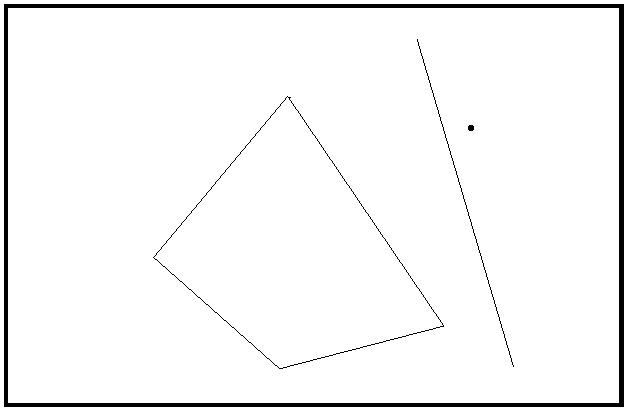
separating hyperplane (see [1], Section 2.4). A sketch of this for the restricted case we have is as
follows. Let y ∈ convexhull(X) minimize the distance from x∗ to convexhull(X). The claim is
that a hyperplane that is normal to the line segment joining x∗ and y and passing through x∗ is
the desired hyperplane. Otherwise convexhull(X) intersects this hyperplane, and let y0 be a point
in the intersection. Since convexhull(X) is convex, the line segment joining y0 and y is contained
in convexhull(X). Now consider the right angled triangle formed by y, x∗, y0. From elementary
geometry, it follows that there is a point closer to x∗ than y on the line segment joining y and y0,
contradicting the choice of y.
2
Now consider max{αx | x ∈ P}. The set of optimal solutions to this LP is a face of F. By
Claim 20, X∩F = ∅. Since F is a face of P, it has a vertex of P since P is pointed. This contradicts
that X is the set of all vertices of P.
2
One consequence of the decomposition theorem is the following.
Theorem 21 If P = {x | Ax ≤ b} is pointed then for any c = 0 the LP
max cx
Ax ≤ b
is either unbounded, or there is a vertex x∗ such that x∗ is an optimal solution.
The proof of the previous theorem is left as an exercise.
2
Complexity of Linear Programming
Recall that LP is an optimization problem of the following form.
max αx
Ax ≤ b
As a computational problem we assume that the inputs c, A, b are rational. Thus the input
consists of n + m × n + n rational numbers. Given an instance I we use size(I) to denote the
number of bits in the binary representation of I. We use it loosely for other quantities such as
numbers, matrices, etc. We have that size(I) for an LP instance is,
size(c) + size(A) + size(b) ≤ (m × n + 2n)size(L)
where L is the largest number in c, A, b.
Lemma 22 Given a n × n rational matrix size(det(A)) = poly(size(A)).
Proof: For simplicity assume that A has integer entries, otherwise one can multiply each entry by
the lcm of the denominators of the rational entries. We have
X
Yn
det(A) =
sign(σ)
Ai,σ(i)
σ∈Sn
i=1
where Sn is the set of all permutations on {1, . . . , n}. Hence
X Yn
|
det(A)| ≤
|Ai,σ(i)|
σ∈S i=1
n
n! × L
n
≤
where L = max |A |; here |x| for a number x is its absolute value. Therefore the number of bits
i,j
required to represent det(A) is O(n log L + n log n) which is polynomial in n and log L, and hence
poly(size(A)).
2
Corollary 23 If A has an inverse, then size(A−1) = poly(size(A)).
Corollary 24 If Ax = b has a feasible solution then there exists a solution x∗ such that size(x∗) =
poly(size(A, b)).
Proof: Suppose Ax = b has a feasible solution. By basic linear algbegra, there is a square submatrix
U of A with full rank and a sub-vector b0
such that −1 0 padded by 0’s for the other variables is
U
b
a feasible solution for the original system. We then apply the previous corollary to U and b0.
2
Gaussian elimination can be adapted using the above to show the following — see [3].
Theorem 25 There is a polynomial time algorith, that given a linear system Ax = b, either
correctly outputs that it has no feasible solution or outputs a feasible solution. Moreover, the
algorithm determines whether A has a unique feasible solution.
Now we consider the case when Ax ≤ b has a feasible solution.
Theorem 26 If a linear system Ax ≤ b has a feasible solution then there exists a solution x∗ such
that size(x∗) = poly(size(A, b)).
Proof: Consider a minimal face F of P = {x | Ax ≤ b}. We have seen that F = {x | A0x =
0
for some subsystem
0
0 of
. By Theorem 25,
0
A x
=
0 has a solution of size
b
b }
A x ≤ b
Ax ≤ b
poly(size(A0, b0)).
2
Corollary 27 The problem of deciding whether {x | Ax ≤ b} is non-empty is in NP.
Corollary 28 The problem of deciding whether {x | Ax ≤ b} is empty is in NP. Equivalently the
problem of deciding non-emptiness is in coNP.
Proof: By Farkas’ lemma, if Ax ≤ b is empty only if ∃y ≥ 0 such that yA = 0 and yb = −1.
Therefore there is a certificate y the problem of deciding whether {x | Ax ≤ b} is empty. Further,
by Lemma 22 this certificate has polynomial size.
2
Thus we have seen that deciding whether Ax ≤ b is non-empty is in NP ∩ coNP.
Now consider the optimization problem.
max αx
Ax ≤ b
A natural decision problem associated with the above problem is to decide if the optimum value
is at least some given rational number α.
Exercise 5 Prove that the above decision problem is in NP ∩ coNP.
Another useful fact is the following.
Theorem 29 If the optimum value of the LP max cx such that Ax ≤ b is finite then the optimum
value has size polynomial in the input size.
Proof:[sketch] If the optimum value is finite then by strong duality then it is achieved by a solution
(x0, y0) that satisfies the following system:
cx = yb
Ax ≤ b
yA = c
y ≥ 0.
From Theorem 26, there is a solution (x∗, y∗) to the above system with size(x∗, y∗) polynomial in
size(A, b, c). Hence the optimum value which is cx∗ has size polynomial in size(A, b, c).
2
Exercise 6 Show that the decision problem of deciding whether max cx where Ax ≤ b is unbounded
is in NP ∩ coNP.
The optimization problem for
max αx
Ax ≤ b
requires an algorithm that correctly outputs one of the following
1
2
3
. Ax ≤ b is infeasible
. the optimal value is unbounded
. a solution x∗ such that cx∗ is the optimum value
A related search problem is given Ax ≤ b either output that Ax ≤ b is infeasible or a solution
such that
x∗
Ax ≤ b
∗
.
Exercise 7 Prove that the above two search problems are polynomial time equivalent.
3
Polynomial-time Algorithms for LP
Khachiyan’s ellipsoid algorithm in 1978 was the first polynomial-time algorithm for LP. Although
an impractical algorithm, it had (and contiues to have) a major theoretical impact. The algorithm
shows that one does not need the full system Ax ≤ b in advance. If one examines carefully the size
of a proof of feasibility of a system of inequalities Ax ≤ b, one notices that there is a solution x∗
such that x∗ is a solution to A0x ≤ b0 for some subsystem A0x ≤ b0 where rank of A is at most n.
This implies that A0 can be chosen to have at most n rows. Therefore, if the system has a solution
then there is one whose size is polynomial in n and the size of the largest entry in A. We may
discuss more details of the ellipsoid method in a later lecture.
Subsequently, Karmarkar in 1984 gave another polynomial-time algorithm using an interior
point method. This is much more useful in practice, especially for certain large linear programs,
and can beat the simplex method which is the dominant method in practice although it is not a
polynomial time algorithm in the worst case.
References
[
[
[
1] S. Boyd and L. Vandenberghe. Convex Optimization. Cambridge University Press, 2004.
Available electronically at http://www.stanford.edu/ boyd/cvxbook/.
2] M. Goemans. Lecture notes on linear programming and polyhedral combinatorics. http:
/www-math.mit.edu/ goemans/18433S09/polyhedral.pdf, 2009.
3] A. Schrijver. Theory of Linear and Integer Programming (Paperback). Wiley, Chapters 7, 8,
998.
1
CS 598CSC: Combinatorial Optimization
Instructor: Chandra Chekuri
Lecture date: 01/28/2010
Scribe: GuoJun Qi
1
Integer Programming, Integer Polyhedra, and Totally Unimod-
ular Matrices
Many discrete optimization problems are naturally modeled as an integer (linear) programming
(ILP) problem. An ILP problem is of the form
max cx
Ax ≤ b
x is an integer vector.
(1)
It is easy to show that ILP is NP-hard via a reduction from say SAT. The decision version of ILP is
the following: Given rational matrix A and rational vector b, does Ax ≤ b have an integral solution
x?
Theorem 1 Decision version of ILP is in NP, and hence it is NP-Complete.
The above theorem requires technical work to show that if there is an integer vector in Ax ≤ b
then there is one whose size is polynomial in size(A, b).
A special case of interest is when the number of variables, n, is a fixed constant but the number
of constraints, m, is part of the input. The following theorem is known.
Theorem 2 (Lenstra’s Algorithm) For each fixed n, there is a polynomial time algorithm for
ILP in n variables.
1
.1 Integer Polyhedra
Given a rational polyhedron P = {x|Ax ≤ b}, we use PI to denote the convex hull of all the integer
vectors in P; this is called the integer hull of P.
It is easy to see that if P is a polytope then PI is also a polytope. Somewhat more involved is
the following.
Theorem 3 For any rational polyhedron P, PI is also a polyhedron.
Definition 4 A rational polyhedron P is an integer polyhedron if and only if P = PI.
Theorem 5 The following are equivalent:
(i) P = PI i.e., P is integer polyhedron.
(ii) Every face of P has an integer vector.
(iii) Every minimal face of P has an integer vector.

(iv) max{cx|x ∈ P} is attained by an integer vector when the optimum value is finite.
Proof: (i)=⇒(ii): Let F be a face, then F = P ∩ H, where H is a supporting hyperplane, and let
x ∈ F. From P = PI, x is a convex combination of integral points in P, which must belong to H
and thus to F.
(ii)=⇒(iii): it is direct from (ii).
(iii)=⇒(iv): Let δ = max{cx : x ∈ P} < +∞, then F = {x ∈ P : cx = δ} is a face of P, which has
an integer vector from (iii).
(iv)=⇒(i): Suppose there is a vector y ∈ P \ PI . Then there is an inequality αx ≤ β valid for PI
while αy > β (a hyperplane separating y and P ). It follows that max{αx | x ∈ P } ≤ β while
I
I
max{αx | x ∈ P} > β since y ∈ P \ PI. Then (iv) is violated for c = α.
2
Another useful theorem that characterizes integral polyhedra, in full generality due to Edmons
and Giles [1977], is the following.
Theorem 6 A rational polyhedron P is integral if and only if max{cx | Ax ≤ b} is an integer for
each integral vector c for which the maximum is finite.
1
.2 Totally Unimodular Matrices
Totally Unimodular Matrices give rise to integer polyhedra with several fundamental applications
in combinatorial optimization.
Definition 7 A matrix A is totally unimodular (TUM) if the determinant of each square submatrix
of A is in {0, 1, −1}. In particular, each entry of A is in {0, 1, −1}.
Proposition 8 If A is TUM and U is a non-singular square submatrix of A, then U−1 is an
integral matrix.
U∗
Proof: U−1 =
where U∗ is the adjoint matrix of U. From the definition of total unimod-
det(U)
ularity, U∗ only contains entries in {0, +1, −1} and det(U) = 1 or −1. Therefore, U is an integral
matrix.
2
Theorem 9 If A is TUM then for all integral b, the polyhedron P = {x|Ax ≤ b} is an integer
polyhedron.
Proof: Consider any minimal face F of P. F = {x|A′x = b′} for some subsystem A′x ≤ b′ of
Ax ≤ b. Let A′ have m′ ≤ n rows. Then A′ = [U V ], where U is a m′ × m′ matrix of full row and
column rank (after potentially rearranging rows and columns). U is a submatrix of A and hence
ꢀ
ꢁ
U−1b′
det(U) ∈ {−1, +1}. Therefore A′x = b′ has an integer solution
. Thus every minimal
0
face has an integer vector and hence P is an integer polyhedron.
We claim several important corollaries.
2
Corollary 10 If A is TUM then for all integral vector a, b, c, d, the polyhedron {x|a ≤ x ≤ b, c ≤
Ax ≤ d} is integral.

I
−I
Proof: If A is TUM, so is the matrix
. This can be easily proven by expanding the
A
−
submatrix along the row associated with the identity matrix.
A
2
Proposition 11 A is TUM ⇐⇒ AT is TUM.
Corollary 12 If A is TUM and b, c are integral vectors, then max{cx|Ax ≤ b, x ≥ 0} = min{yb|yA ≤
c, y ≥ 0} are attained by integral vectors x∗ and y∗, if they are finite.
ꢂ
ꢃ
AT
Proof: The polyhedron {y|y ≥ 0, yA ≤ c} is integral since AT is TUM and also
.
2
−
I
There are many characterizations of TUM matrices. We give a few useful ones below. See [1]
(Chapter 19) for a proof.
Theorem 13 Let A be a matrix with entries in {0, +1, −1}. Then the followings are equivalent.
(i) A is TUM.
(ii) For all integral vector b, {x|Ax ≤ b, x ≥ 0} has only integral vertices.
(iii) For all integral vectors a, b, c, d, {x|a ≤ x ≤ b, c ≤ Ax ≤ d} has only integral vertices.
(iv) Each collection of column S of A can be split into two sets S and S such that the sum of
1
2
columns in S minus the sum of columns in S is a vector with entries in {0, +1, −1}.
1
2
(v) Each nonsingular submatrix of A has a row with an odd number of nonzero components.
(vi) No square submatrix of A has determinant +2 or −2.
(i) ⇐⇒ (ii)is the Hoffman-Kruskal’s theorem. (ii) =⇒ (iii) follows from the fact that A is TUM
I
−I
=
⇒
is TUM. (i) ⇐⇒ (iv) is Ghouila-Houri’s theorem.
A
−
Several important matrices that arise in combinatorial optimization are TUM.
A
Example 1: Bipartite Graphs. Let G = (V, E) an undirected graph. Let M be the {0, 1}
edge-vetex incidence matrix defined as follows. M has |E| rows, one for each edge and |V | columns,
one for each vertex. Me,v = 1 if e is incident to v otherwise it is 0. The claim is that M is TUM
iff G is bipartite.
0
1 1
To see bipartiteness is needed, consider the matrix 1 0 1 for a triangle which is an odd
1
1 0
cycle. Its determinant is 2.
Exercise 1 Show that edge-vertex adjacency matrix of any odd cycle has determinant 2.
a1
a’2
a2
a’3
a’1
a4
a3
Figure 1: Network matrix is defined by a directed tree (dotted edges) and a directed graph on the
same vertex set.
Example 2: Directed Graphs. Let D = (V, A) be a directed graph. Let M be an |E| × |V |
arc-vertex adjacency matrix defined as
0
, if a is not incident to v
+1, if a enters v
1, if a leaves v
Ma,v
=
(2)
−
M is TUM. This was first observed by Poincare´ [1900].
Example 3: Consecutive 1’s: A is a consecutive 1’s matrix if it is a matrix with entries in
0, 1} such that in each row the 1’s are in a consecutive block. This naturally arises as an incidence
{
matrix of a collection of intervals and a set of points on the real line.
The above three claims of matrices are special cases of network matrices (due to Tutte).
Definition 14 A network matrix is defined from a directed graph D = (V, A) and a directed tree
T = (V, A′) on the same vertex set V . The matrix M is |A′|×|A| matrix such that for a = (u, v) ∈ A
and a′ ∈ A′
0
, if the unique path from u → v in T does not contain a′
+1, if the unique path from u → v in T passes through a′ in forward direction
1, if the unique pathu → v in T passes through a′ in backward direction
Ma,a′
=
−
The network matrix corresponding to the directed graph and the tree in Figure 1 is given below.
The dotted edge is T, and the solid edge is D.
a1 a2 a3 a4
−1 1
a′
1
0
−1 −1
1
M = a′
0
−1 1
0
2
a′
3
0
1
Theorem 15 (Tutte) Every network matrix is TUM.
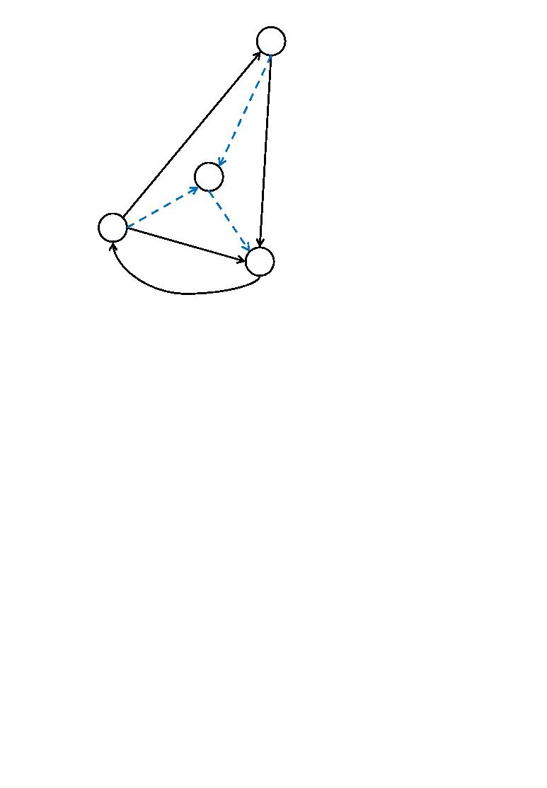
u
(a)
(b)
Figure 2:
We will prove this later. First we show that the previous examples can be cast as special cases of
network matrices.
Bipartite graphs. Say G = {X ∪Y, E} as in Figure 2(a). One can see that edge-vertex adjacency
matrix of G as the network matrix induced by a directed graph G = (X ∪ Y ∪ {u}, A) where
u is a new vertex and A is the set of arcs defined by orientating the edges of G from X to Y .
T = (X ∪ Y ∪ {u}, A′) where A′ = {(v, u)|v ∈ X} ∪ {(u, v)|v ∈ Y } as in Figure 2(b).
Directed graphs. Suppose D = (V, A) is a directed graph. Consider the network matrix induced
by D = (V ∪{u}, A) and T = (V ∪{u}, A′) where u is a new vertex and where A′ = {(v, u)|v ∈ V }.
Consecutive 1’s matrix. Let A be a consecutive 1’s matrix with m rows and n columns. Assume
for simplicity that each row has at least one 1 and let ℓ and r be the left most and right most
i
i
columns of the consecutive block of 1’s in row i. Let V = {1, 2, . . . , n}. Consider T = (V, A′) where
A′ = {(i, i + 1) | 1 ≤ i < n} and D = (V, A) where A = {(ℓ , r ) | 1 ≤ i ≤ n}. It is easy to see that
i
i
A is the network matrix defined by T and A.
Now we prove that every network matrix is TUM. We need a preliminary lemma.
Lemma 16 Every submatrix M′ of a network matrix M is also a network matrix.
Proof: If M is a network matrix, defined by D = (V, A) and T = (V, A′), then removing a column in
M corresponds to removing an arc a ∈ A. Removing a row corresponds to identifying/contracting
the end points of an arc a′ in T.
2
Proposition 17 A is TUM ⇐⇒ A′ obtained by multiplying any row or column by −1 is TUM.
Corollary 18 If M is a network matrix, M is TUM ⇐⇒ M′ is TUM where M′ is obtained by
reversing an arc of either T or D.
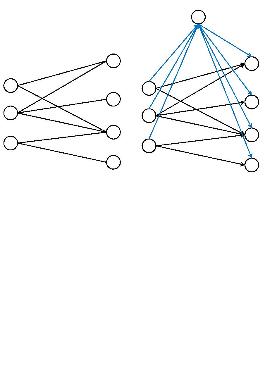
v
v
a1
a1
(v,w)
u
u
a2
w
w
Before subtracting a1 from a2
After subtracting a1 from a2
Edges in directed graph
Edges in associated tree
Figure 3:
Proof of Theorem 15. By Lemma 16, it suffices to show that any square network matrix C
has determinant in {0, +1, −1}. Let C be a k × k network matrix defined by D = (V, A) and
T = (V, A′). We prove by induction on k that det(C) ∈ {0, 1, −1}. Base case with k = 1 is trivial
since entries of C are in {0, 1, −1}.
Let a′ ∈ A′ be an arc incident to a leaf u in T. By reorienting the arcs of T, we will assume
that a′ leaves u and moreover all arcs A incident to u leave u (see Corollary 18).
Let a , a , · · · , a be arcs in A leaving u (If no arcs are incident to u then det(C) = 0). Assume
1
2
h
without loss of generality that a′ is the first row of C and that a , a , · · · , a are the first h columns
1
2
h
of C.
Claim 19 Let C′ be obtained by subtracting column a from column a . C′ is the network matrix
1
2
for T = (V, A′) and D = (V, A − a + (v, w)) where a = (u, v) and a = (u, w).
2
1
2
We leave the proof of the above as an exercise — see Figure 3.
Let C′′ be the matrix obtained by subtracting column of a from each of a , · · · , a . From
1
2
h
the above claim, it is also a network matrix. Moreover, det(C′′) = det(C) since determinant is
preserved by these operations. Now C′′ has 1 in the first row in column one ( corresponding to a1)
and 0’s in all other columns. Therefore, det(C′′) ∈ {0, +1, −1} by expanding along the first row
and using induction for the submatrix of C′′ consisting of columns 2 to k and rows 2 to k.
2
Some natural questions on TUM matrices are the following.
(i) Are there TUM matrices that are not a network matrix (or its transpose)?
(ii) Given a matrix A, can one check efficiently whether it is a TUM matrix?
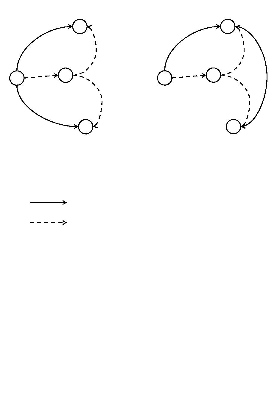
The answer to (i) is negative as shown by the following two matrices given by Hoffman[1960]
1
−1
0
−1
1
−1
0
0
−1
1
−1
0
0
0
−1
0
−1
1
−1 0
0
1
−1
−
1
0
and Bixby[1977].
1
1
1 1 1
1
1 1 0 0
0 0 1 −1
1 0 1 1 0
1
1
1 0 0
1
Amazingly, in some sense, these are the only two exceptions.
Seymour, in a deep and difficult technical theorem, showed via matroid theory methods that any
TUM matrix can be obtained by “gluing” together network matrices and the above two matrices
via some standard operations that preserve total unimodularity. His descomposition theorem also
led to a polynomial time algorithm for checking if a given matrix is TUM. There was an earlier
polynomial time algorithm to check if a given matrix is a network matrix. See [1] (Chapters 20 and
21) for details.
References
[1] A. Schrijver. Theory of Linear and Integer Programming (Paperback). Wiley, 1998.
CS 598CSC: Combinatorial Optimization
Instructor: Chandra Chekuri
Lecture date: Feb 2, 2010
Scribe: Siva Theja Maguluri
Material taken mostly from [1] (Chapter 19).
1
Integer Decomposition Property
A polyhedron P has the integer decomposition property if ∀ integers k ≥ 1 and x ∈ P, kx is integral
implies kx = x + x + . . . + x for integral vectors x , . . . , x in P. Baum and Trotter showed the
1
2
k
1
k
following:
Theorem 1 (Baum and Trotter) A matrix A is TUM iff P = {x | x ≥ 0, Ax ≤ b} has the
integer decomposition property for all integral verctors b.
Proof: We show one direction, the one useful for applications. Suppose A is TUM, consider
P = {x | x ≥ 0, Ax ≤ b}. Let y = kx
∗
be an integral vector where
x ∈ P
∗
. We prove by induction
on k that y = x + x + . . . .x for integral vectors x , x , . . . , x in P.
1
2
k
1
2
k
Base case for k = 1 is trivial.
For k ≥ 2, consider the polyhedron P0 = {x | 0 ≤ x ≤ y; Ay − kb + b ≤ Ax ≤ b}. P0 is an
integral polyhedron since A is TUM and Ay − kb + b and b are integral. The vector x∗ ∈ P0 and
hence P0 is not empty. Hence there is an integral vector x ∈ P0. Moreover y0 = y − x is integral
1
1
and y0 ≥ 0, Ay0 ≤ (k − 1)b.
By induction y0 = x +. . .+x
where x2, . . . , xk−1 are integral vectors in P. y = x1 +. . .+xk
2
k−1
is the desired combination for y.
2
Remark 2 A polyhedron P may have the integer decomposition property even if the constraint
matrix A is not TUM. The point about TUM matrices is that the property holds for all integral
right hand side vectors b.
2
Applications of TUM Matrices
We saw that network matrices are TUM and that some matrices arising from graphs are network
matrices. TUM matrices give rise to integral polyhedra, and in particular, simultaneously to the
primal and dual in the following when A is TUM and c, b are integral vectors.
max{cx | x ≥ 0, Ax ≤ b} = min{yb | y ≥ 0, yA ≥ c}
We can derive some min-max results and algorithms as a consequence.

2
.1 Bipartite Graph Matchings
Let G = (V, E) be a bipartite graph with V = V ⊕ V as the bipartition. We can write an integer
1
2
program for the maximum cardinality matching problem as
X
max
x(e)
e∈E
x(δ(u)) ≤ 1 ∀u ∈ V
x(e) ≥ 0 ∀e ∈ E
x ∈ Z
We observe that this is a ILP problem max{1·x | Mx ≤ 1, x ≥ 0, x ∈ Z} where M is the edge-vertex
incidence matrix of G. Since M is TUM, we can drop the integrality constraint and solve the linear
program max{1 · x | Mx ≤ 1, x ≥ 0} since {x | Mx ≤ 1, x ≥ 0} is an integral polyhedron. The dual
of the above LP is
X
min
y(u)
u∈V
y(u) + y(v) ≥ 1 uv ∈ E
y ≥ 0
in other words min{y · 1|yM ≥ 1, y ≥ 0} which is is also an integral polyhedron since MT is TUM.
We note that this is the min-cardinality vertex cover problem
Note that the primal LP is a polytope and hence has a finite optimum solution. By duality, and
integrality of the polyhedra, we get that both primal and dual have integral optimum solutions x∗
and y∗ such that 1 · x∗ = y∗ · 1. We get as an immediate corollary K¨onig’s Theorem.
Theorem 3 In a bipartite graph the cardinality of a maximum matching is equal to the cardinality
of a minimum vertex cover.
Also, by poly-time solvability of linear programming, there is a polynomial time algorithm for
maximum matching and minimum vertex cover in bipartite graphs, and also their weighted versions.
Note that we have much more efficient combinatorial algorithms for these problems. We also obtain
that {x | Mx ≤ 1, x ≥ 0} is the convex hull of the characteristic vectors of the matchings in G and
that {x | Mx = 1, x ≥ 0} is the convex hull of the perfect matchings of G.
One easy consequence is the following theorem
Theorem 4 (Birkhoff - Von Neumann) Let A be a n × n doubly stochastic matrix. Then A
can be written as a convex combination of permutation matrices.
A doubly stochastic matrix is a square non-negative matrix in which each row and column sum
is 1. A permutation matrix is a square {0, 1} matrix that has a single 1 in each row and column.
Each permulation matrix corresponds to a permutation σ in S , the set of all permutations on an
n
n-element set.
Exercise 5 Prove the above theorem using the perfect matching polytope description for bipartite
graphs. How many permutations matrices do you need in the convex combination?
Note that max{wx | Mx ≤ 1, x ≥ 0} = min{y · 1 | yM ≥ w, y ≥ 0} has integer primal and
dual solutions x∗ and y∗ · 1 if w is integral. For the primal x∗ corresponds to a maximum w-weight
matching. In the dual, via complementary slackness, we have
y u y v w v
∗( ) + ∗( ) = ∗( )
for all x∗(uv) > 0 Interpreting y∗(u) as a weight on u, one obtains a generalization of K¨onig’s
theorem, known as the Egervary theorem.
Another theorem on bipartite graphs is the Hall’s marriage theorem.
Theorem 6 (Hall) Let G = (V, E) be a bipartite graph with X, Y as the vertex sets of the bipar-
tition. Then there is a matching that saturates X iff |N(S)| ≥ |S|∀S ⊆ X where N(S) is the set of
neighbors of S.
Exercise 7 Derive Hall’s theorem from Ko¨nig’s Theorem.
A generalization of the above also holds.
Theorem 8 Let G = (X ∪ Y, E) be a bipartite graph. Let R ⊆ U. Then there is a matching
that covers R iff there exists a matching M that covers R ∩ X and a matching that covers R ∩ Y .
Therefore, a matching covers R iff |N(S)| ≥ |S|∀S ⊆ R ∩ X and ∀S ⊆ R ∩ Y .
Exercise 9 Prove above theorem.
b-matchings: b-matchings generalize matchings. Given an integral vector b : V → Z+
, a -
b
matching is a set of edges such that the number of edges incident to a vertex v is at most b(v).
From the fact that the matrix M is TUM, one can obtain various properties of b-matchings by
observing that the polyhedron
Mx ≤ b
x ≥ 0
is integral for integral b.
2
.2 Single Commodity Flows and Cuts
We can derive various useful and known facts about single commodity flows and cuts using the fact
that the directed graph arc-vertex incidence matrix is TUM.
Consider the s-t maximum-flow problem in a directed graph D = (V, A) with capacities c : A →
R+. We can express the maximum flow problem as an LP with variables x(a) for flow on arc a.
X
X
max
x(a) −
x(a) −
x(a)
a∈δ+(s)
a∈δ−(s)
X
X
x(a) = 0 ∀v ∈ V − {s, t}
a∈δ+(v)
a∈δ−(v)
x(a) ≤ c(a) ∀a ∈ A
x(a) ≥ 0 ∀a ∈ A
Note that the polyhedron defined by the above is of the form {x | M0x = 0, 0 ≤ x ≤ c} where
is the arc-vertex incidence matrix of with the columns corresponding to removed.
M0
D
s, t
M
0
is a submatrix of M, the arc-vertex incidence matrix of D which is TUM, and hence M0 is also
TUM. Therefore, the polyhedron above is integral for integral c. One immediate corollary is that
for integral capacities, there is a maximum flow that is integral. We now derive the maxflow-mincut
theorem as a consequence of the total unimodularity of M.
The dual to the maximum-flow LP above has two sets of variables. y(a), a ∈ A for the capacity
constraints and z(v), v ∈ V −{s, t} for the flow conservation constraints. We let w(a) be the weight
vector of the primal. Note that
1
if a = (s, v) for some v ∈ V
if a = (v, s) for some v ∈ V
otherwise
w(a) =
1
−
0
For simplicity assume that there is no arc (s, t) or (t, s). Then the dual is:
X
min
c(a)y(a)
a∈A
z(u) − z(v) + y(u, v) ≥ 0
(u, v) ∈ A {u, v} ∩ {s, t} = ∅
z(v) + y(s, v) ≥ 1 ∀(s, v) ∈ A
z(v) + y(s, v) ≥ −1 ∀(v, s) ∈ A
z(v) + y(v, t) ≥ 0 ∀(v, t) ∈ A
−
z(v) + y(t, v) ≥ 0 ∀(t, v) ∈ A
y ≥ 0
Note that z are unconstrained variables. In matrix form, the primal is max{wx | M0x = 0, 0 ≤
x ≤ c} and the dual is min{yc | y ≥ 0; ∃z : y + zM ≥ w }
0
T . Since is integral and 0 is TUM,
w
M
dual is an integral polyhedron. Primal is bounded polyhedron and hence primal and dual have
optimal solution x∗ and (y∗, z∗) such that wx∗ = y∗c and y∗, z∗ is integral.
We can extend z to have variables z(s) and z(t) with z(s) = −1 and z(t) = 0. Then the dual has
a cleaner form, max{yc | y ≥ 0, ∃z : y +zM ≥ 0}. Note that M here is the full arc-vertex incidence
matrix of D. Thus we have x∗ and integral (y∗, z∗) such that wx∗ = y∗c and y∗ + z∗M ≥ 0.
Let U = {v ∈ V |z∗(v) < 0}. Note that s ∈ U and t ∈/ U and hence δ+(U) is a s-t cut.
P
Claim 10 c(δ+(U)) ≤ y∗c =
y∗(a)c(a)
a∈A
Proof: Take any arc (u, v) ∈ δ+(U). We have z∗(u) − z∗(v) + y∗(u, v) ≥ 0 for each (u, v). Since
u ∈ U and v ∈/ U, z u <
∗
( ) 0 and ∗( ) 0. Since ∗ is integral, we have
z v ≥
z
∗
y u, v
(
)
1
≥
X
=
⇒ c(δ+(U)) ≤
c(a)y∗(a)
a∈δ+(U)
X
c(a)y (a) since
∗
y∗ ≥
0
≤
a∈A
2
Therefore, U is a s-t cut of capacity at most y∗c = wx∗ but wx∗ is the value of a maximum
flow. Since the capacity of any cut upper bounds the maximum flow, we have that there exists a
cut of capacity equal to that of the maximum flow. We therefore, get the following theorem,
Theorem 11 In any directed graph G = (V, A) with non-negative arc capacities, c : E → Q+, the
s-t maximum-flow value is equal to the s-t minimum cut capacity. Moreover, if c : E → z
+
, then
there is an integral maximum flow.
Interpretation of the dual values: A natural interpretation of the dual is the following. The
dual values, y(a) indicate whether a is cut or not. The value z(v) is the shortest path distance
from s to v with y(a) values as the length on the arcs. We want to separate s from t. So, we have
(implicitly) z(s) = −1 and z(t) = 0. The constraints z(u) − z(v) + y(u, v) ≥ 0 enforce that the z
P
values are indeed shortest path distances. The objective function
c(a)y(a) is the capacity of the
a∈A
cut subject to separating s from t.
Circulations and lower and upper bounds on arcs: More general applications of flows are
obtained by considering both lower and upper bounds on the flow on arcs. In these settings,
circulations are more convenient and natural.
Definition 12 For a directed graph D = (V, A), a circulation is a function f : A → R+ such that
P
P
f(a) =
f(a)∀v ∈ V
a∈δ−(v)
a∈δ+(v)
Given non-negative lower and upper bounds on the arcs, l : A → R+ and u : A → R+, we are
interested in circulations that satisfy the bounds on the arcs. In other words, the feasibility of the
following:
l(a) ≤ x(a) ≤ u(a)
x is a circulation
The above polyhedron is same as {x | Mx = 0, l ≤ x ≤ u} where M is the arc-vertex incidence
graph of D, which is TUM. Therefore, if l, u are integral then the polyhedron is integral. Checking
if there is a feasible circulation in a graph with given l and u is at least as hard as solving the
maximum flow problem.
Exercise 13 Given D, s, t ∈ V and a flow value F, show that checking if there is an s − t flow of
value F can be efficently reduced to checking if a given directed graph has a circulation respecting
lower and upper bounds.
The converse is also true however; one can reduce circulation problems to regular maximum-flow
problems, though it takes a bit of work.
Min-cost circulation is the problem: min{cx | l ≤ x ≤ u, Mx = 0}. We therefore obtain that
Theorem 14 The min-cost circulation problem with lower and upper bounds can be solved in
(strongly) polynomial time. Moreover, if l, u are integral then there exists an integral optimum
solution.
The analogue of max flow-min cut theorem in the circulation setting is Hoffman’s circulation
theorem.
Theorem 15 Given D = (V, A) and l : A → R+ and u : A → R+, there is a feasible circulation
iff
x : A → R
+
1
. l(a) ≤ c(a) ∀a ∈ A and
2
. ∀U ⊆ V, l(δ−(U)) ≤ c(δ+(U)).
Moreover, if l, u are integral then there is an integral circulation.
Exercise 16 Prove Hoffman’s theorem using TUM property of M and duality.
b-Transshipments: One obtains slightly more general objects called transshipments as follows:
Definition 17 Let D = (V, E) be a directed graph and b : A → R. A b-transshipment is a function
f : A → R
b(u).
+
such that ∀ ∈
u
V f δ
,
( −( )) − ( +( )) = ( ) i.e, the excess inflow at is equal to
u
f δ
u
b u
u
We think of nodes u with b(u) < 0 as supply nodes and b(u) > 0 as demand nodes. Note that
b = 0 captures circulations. Once can generalize Hoffman’s circulation theorem.
Theorem 18 Given D = (V, A), b : V → R+ and l : A → R+and u : A → R+,there exists a
b-transshipment respecting l, u iff
1
2
. l(a) ≤ u(a) ∀a ∈ A and
P
.
b(v) = 0 and
v∈V
3
. ∀S ⊆ V , u(δ+(S)) ≥ l(δ−(S)) + b(S).
Moreover, if b, l, u are integral, there is an integral b-transshipment.
Exercise 19 Derive the above theorem from Hoffman’s circulation theorem.
2
.3 Interval graphs
A graph G = (V, E) on n nodes is an interval graph if there exist a collection I of n closed intervals
on the real line and a bijection f : V → I such that uv ∈ E iff f(u) and f(v) intersect. Given an
interval graph, an interesting problem is to find a maximum weight independent set in G where
is a weight function. This is same as asking for the maximum weight non-overlapping
w : A → R+
set of intervals in a collection of intervals.
We can write an LP for it. Let I = {I , . . . , I }
1
n
Xn
max
wixi
i=1
X
xi ≤ 1 ∀p in R
I :p∈I
i
i
xi ≥ 0
1 ≤ i ≤ n
Note that the constraints can be written only for a finite set of points which correspond to the
end points of the intervals. These are the natural “clique” constraints: each maximal clique in G
corresponds to a point p and all the intervals containing p. and clearly an independent set cannot
pick more than one node from a clique.
The LP above is max{wx | x ≥ 0, Mx ≤ 1} where M is a consecutive ones matrix, and hence
TUM. Therefore, the polyhedron is integral. We therefore have a polynomial time algorithm for
the max-weight independent set problem in interval graphs. This problem can be easily solved
efficienctly via dynamic programming. However, we observe that we can also solve max{wx|x ≥
0
, Mx ≤ b}for any integer b and this is not easy to see via other methods.
To illustrate the use of integer decomposition properties of polyhedra, we derive a simple and
well known fact.
Proposition 20 Suppose we have a collection of intervals I such that ∀p ∈ R the maximum
number of intervals containing p is at most k. Then I can be partitioned into I , I , . . . , I such
1
2
k
that each I is a collection of non-overlapping intervals. In other words, if G is an interval graph
k
then ω(G) = χ(G) where ω(G) is the clique-number of G and χ(G) is the chromatic number of G.
One can prove the above easily via a greedy algorithm. We can also derive this by considering
the independent set polytope {x | x ≥ 0, Mx ≤ 1}. We note that x∗ = 1 .1 is feasible for this
k
polytope if no point p is contained in more than k intervals. Since P has the integer decomposition
property, y = kx∗ = 1 can be written as x + . . . + x where x is integral ∀1 ≤ i ≤ k and x ∈ P.
1
k
i
i
This gives the desired decomposition. The advantage of the polyhedral approach that one obtains
a more general theorem by using an arbitrary integral b in the polytope {x | x ≥ 0, Mx ≤ b} and
this has applications; see for example [2].
References
[
[
1] A. Schrijver. Theory of Linear and Integer Programming (Paperback). Wiley, 1998.
2] P. Winkler and L. Zhang. Wavelength Assignment and Generalized Interval Graph Coloring.
ACM-SIAM SODA, 2003.

CS 598CSC: Combinatorial Optimization
Instructor: Chandra Chekuri
Lecture date: 2/4/2010
Scribe: David Morrison
Gomory-Hu Trees
(The work in this section closely follows [3])
Let G = (V, E) be an undirected graph with non-negative edge capacities defined by c : E → R.
We would like to be able to compute the global minimum cut on the graph (i.e., the minimum
over all min-cuts between pairs of vertices s and t). Clearly, this can be done by computing the
ꢀ
ꢁ
minimum cut for all n pairs of vertices, but this can take a lot of time. Gomory and Hu showed
2
that the number of distinct cuts in the graph is at most n − 1, and furthermore that there is an
efficient tree structure that can be maintained to compute this set of distinct cuts [1] (note that
there is also a very nice randomized algorithm due to Karger and Stein that can compute the global
minimum cut in near-linear time with high probability [2]).
An important note is that Gomory-Hu trees work because the cut function is both submodular
and symmetric. We will see later that any submodular, symmetric function will induce a Gomory-
Hu tree.
Definition 1. Given a graph G = (V, E), we define αG(u, v) to be the value of a minimum u, v
cut in G. Furthermore, for some set of vertices U, we define δ(U) to be the set of edges with one
endpoint in U.
Definition 2. Let G, c, and αG be defined as above. Then, a tree T = (V (G), ET ) is a Gomory-
Hu tree if for all st ∈ E , δ(W) is a minimum s, t cut in G, where W is one component of
T
T − st.
The natural question is whether such a tree even exists; we will return to this question shortly.
However, if we are given such a tree for an arbitrary graph G, we know that this tree obeys some
very nice properties. In particular, we can label the edges of the tree with the values of the minimum
cuts, as the following theorem shows (an example of this can be seen in figure 1):
Theorem 1. Let T be a Gomory-Hu tree for a graph G = (V, E). Then, for all u, v ∈ V , let st be
the edge on the unique path in T from u to v such that α (s, t) is minimized. Then,
G
α (u, v) = α (s, t)
G
G
and the cut δ(W) induced by T − st is a u, v minimum cut in G. Thus α (s, t) = α (s, t) for each
G
T
s, t ∈ V where the capacity of an edge st in T is equal to α (s, t).
G
Proof. We first note that α obeys a triangle inequality. That is, α (a, b) ≥ min(α (a, c), α (b, c))
G
G
G
G
for any undirected graph G and vertices a, b, c (to see this, note that c has to be on one side or the
other of any a, b cut).
Consider the path from u to v in T. We note that if uv = st, then α (u, v) = α (s, t).
G
G
Otherwise, let w = v be the neighbor of u on the u-v path in T. By the triangle inequality
mentioned above, α (u, v) ≥ min(α (u, w), α (w, v)). If uw = st, then α (u, v) ≥ α (s, t);
G
G
G
G
G
otherwise, by induction on the path length, we have that α (u, v) ≥ α (w, v) ≥ α (s, t).
G
G
G
However, by the definition of Gomory-Hu trees, we have that α (u, v) ≤ α (s, t), since the cut
G
G
induced by T − st is a valid cut for u, v. Thus, we have α (u, v) = α (s, t) and the cut induced by
G
G
T − st is a u, v minimum cut in G.
ꢀ

4
b
c
5
7
1
0
2
2
a
3
d
1
8
17
13
15
a
b
f
e
c
8
3
f
e
1
4
2
d
Figure 1: A graph G with its corresponding Gomory-Hu tree [4].
Remark 2. Gomory-Hu trees can be (and are often) defined by asking for the property described in
Theorem 1. However, the proof shows that the basic requirement in Definition 2 implies the other
property.
The above theorem shows that we can represent compactly all of the minimum cuts in an
undirected graph. Several non-trivial facts about undirected graphs fall out of the definition and
the above result. The only remaining question is “Does such a tree exist? And if so, how does one
compute it efficiently?” We will answer both questions by giving a constructive proof of Gomory-Hu
trees for any undirected graph G. However, first we must discuss some properties of submodular
functions.
Definition 3. Given a finite set E, f : 2E → R is submodular if for all A, B ∈ 2E, f(A)+f(B) ≥
f(A ∪ B) + f(A ∩ B).
An alternate definition based on the idea of “decreasing marginal value” is the following:
Definition 4. Given E and f as above, f is submodular if f(A + e) − f(A) ≥ f(B + e) − f(B) for
all A ⊆ B and e ∈ E.
To see the equivalence of these definitions, let f (e) = f(A+e)−f(A), and similarly for f (e).
A
B
Take any A, B ⊆ E and e ∈ E such that A ⊆ B, and let f be submodular according to definition 3.
Then f(A + e) + f(B) ≥ f((A + e) ∪ B) + f((A + e) ∩ B) = f(B + e) + f(A). Rearranging shows
that f (e) ≥ f (e). Showing that definition 4 implies definition 3 is slightly more complicated, but
A
B
can be done (Exercise).
There are three types of submodular functions that will be of interest:
1
2
. Arbitrary submodular functions
. Non-negative (range is [0, ∞)). Two subclasses of non-negative submodular functions are
monotone (f(A) ≤ f(B) whenever A ⊆ B) and non-monotone.
3
. Symmetric submodular functions where f(A) = f(E \ A) for all A ⊆ E.
As an example of a submodular function, consider a graph G = (V, E) with capacity function
c : E → R
+
. Then : 2V R+ defined by ( ) = ( ( )) (i.e., the capacity of a cut induced by a
f
to f A
c δ A
set A) is submodular.
To see this, notice that f(A) + f(B) = a + b + 2c + d + e + 2f, for any arbitrary A and B, and
a, b, c, d, e, f are as shown in figure 2. Here, a (for example) represents the total capacity of edges
with one endpoint in A and the other in V \ (A ∪ B). Also notice that f(A ∪ B) + f(A ∩ B) =
a+b+2c+d+e, and since all values are positive, we see that f(A)+f(B) ≥ f(A∪B)+f(A∩B),
satisfying definition 3.
a
b
c
e
A
d
B
f
Figure 2: Given a graph G and two sets A, B ⊆ V , this diagram shows all of the possible classes
of edges of interest in G. In particular, there could be edges with both endpoints in V \ (A ∪ B),
A, or B that are not shown here.
Exercise 1. Show that cut function on the vertices of a directed graph is submodular.
Another nice property about this function f is that it is posi-modular, meaning that f(A) +
f(B) ≥ f(A − B) + f(B − A). In fact, posi-modularity follows for any symmetric submodular
function:
f(A) + f(B) = f(V − A) + f(B) ≥ f ((V − A) ∩ B) + f ((V − A) ∪ B)
=
=
f(B − A) + f (V − (A − B))
f(B − A) + f(A − B)
We use symmetry in the first and last lines above. In fact, it turns out that the above two
properties of the cut function are the only two properties necessary for the proof of existence of
Gomory-Hu trees. As mentioned before, this will give us a Gomory-Hu tree for any non-negative
symmetric submodular function. We now prove the following lemma, which will be instrumental
in constructing Gomory-Hu trees:
Key Lemma. Let δ(W) be an s, t minimum cut in a graph G with respect to a capacity function
c. Then for any u, v ∈ W, u = v, there is a u, v minimum cut δ(X) where X ⊆ W.
Proof. Let δ(X) be any u, v minimum cut that crosses W. Suppose without loss of generality that
s ∈ W, s ∈ X, and u ∈ X. If one of these are not the case, we can invert the roles of s and t or X
and V \ X. Then there are two cases to consider:
Case 1: t ∈ X (see figure 3). Then, since c is submodular,
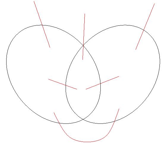
X
t
u
s
W
v
Figure 3: δ(W) is a minimum s, t cut. δ(X) is a minimum u, v cut that crosses W. This diagram
shows the situation in Case 1; a similar picture can be drawn for Case 2
c(δ(X)) + c(δ(W)) ≥ c(δ(X ∩ W)) + c(δ(X ∪ W))
(1)
But notice that δ(X∩W) is a u, v cut, so since δ(X) is a minimum cut, we have c(δ(X∩W)) ≥
c(δ(X)). Also, X ∪ W is a s, t cut, so c(δ(X ∪ W)) ≥ c(δ(W)). Thus, equality holds in
equation (1), and X ∩ W is a minimum u, v cut.
Case 2: t ∈ X. Since c is posi-modular, we have that
c(δ(X)) + c(δ(W)) ≥ c(δ(W \ X)) + c(δ(X \ W))
(2)
However, δ(W \ X) is a u, v cut, so c(δ(W \ X)) ≥ c(δ(X)). Similarly, δ(X \ W) is an s, t
cut, so c(δ(X \ W)) ≥ c(δ(W)). Therefore, equality holds in equation (2), and W \ X is a
u, v minimum cut.
ꢀ
The above argument shows that minimum cuts can be uncrossed, a technique that is useful in
many settings. In order to construct a Gomory-Hu tree for a graph, we need to consider a slightly
generalized definition:
Definition 5. Let G = (V, E), R ⊆ V . Then a Gomory-Hu tree for R in G is a pair consisting
of T = (R, E ) and a partition (C | r ∈ R) of V associated with each r ∈ R such that
T
r
1
. For all r ∈ R, r ∈ Cr
2
. For all st ∈ ET , T − st induces a minimum cut in G between s and t defined by
[
δ(U) =
Cr
r∈X
where X is the vertex set of a component of T − st.
Notice that a Gomory-Hu tree for G is simply a generalized Gomory-Hu tree with R = V .
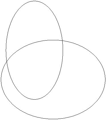
Algorithm 1 GomoryHuAlg(G, R)
if |R| = 1 then
return T = ({r}, ∅), C = V
r
else
Let r , r ∈ R , and let δ(W) be an r , r minimum cut
1
2
1
2
hhCreate two subinstances of the problemii
G = G with V \ W shrunk to a single vertex, v ; R = R ∩ W
1
1
1
G = G with W shrunk to a single vertex, v ; R = R \ W
2
2
2
hhNow we recurseii
T , (C
1
r
|
|
r
r
∈
∈
R
) =
) =
GomoryHuAlg G , R
(
)
)
1
1
1
GomoryHuAlg G , R
1
T2, (Cr
2
R2
(
2
2
0
00
hhNote that r , r are not necessarily r , r !ii
1
2
Let r0 be the vertex such that v ∈ C1
1
0
r
Let r00 be the vertex such that v ∈ C2
2
00
r
hhSee figure 4ii
T = (R ∪ R , E ∪ E ∪ {rr }
0
)
1
2
T
T
2
1
(C | r ∈ R) = ComputePartitions(R , R , C1, C2, r0, r00)
r
1
2
r
r
return T, Cr
end if
Algorithm 2 ComputePartitions(R , R , C1, c2, r0, r00)
1
2
r
r
hhWe use the returned partitions, except we remove v and v from C and Cr00 , respectivelyii
1
2
r0
For r ∈ R , r = r0, C = C1
1
r
r
For r ∈ R , r = r00, C = C2
1
r
r
C = C
1
− { }
v , C
=
C
2 − { }
v
2
r0
1
r00
r
0
r
00
return (C | r ∈ R)
r
Intuitively, we associate with each vertex v in the tree a “bucket” that contains all of the
vertices that have to appear on the same side as v in some minimum cut. This allows us to define
the algorithm GomoryHuAlg.
Theorem 3. GomoryHuAlg returns a valid Gomory-Hu tree for a set R.
Proof. We need to show that any st ∈ E satisfies the “key property” of Gomory-Hu trees. That
T
is, we need to show that T − st induces a minimum cut in G between s and t. The base case
is trivial. Then, suppose that st ∈ T or st ∈ T . By the Key Lemma, we can ignore all of the
1
2
vertices outside of T or T , because they have no effect on the minimum cut, and by our induction
1
2
hypothesis, we know that T and T are correct.
1
2
Thus, the only edge we need to care about is the edge we added from r0 to r00. First, consider
the simple case when α (r , r ) is minimum over all pairs of vertices in R. In this case, we see that
G
1
2
in particular, α (r , r ) ≤ α (r0, r00), so we are done.
G
1
2
G
However, in general this may not always be the case. Let δ(W) be a minimum cut between r1
and r2, and suppose that there is a smaller r0, r00 minimum cut δ(X) than what W induces; that
is c(δ(X)) < ¸(δ(W)). Assume without loss of generality that r , r0 ∈ W. Notice that if r ∈ X, we
1
1






T1
T2
r2
r’
C = {v ,...}
r’’
1
r’
2
C = {v ,...}
r’’
1
2
r1
Figure 4: T and T have been recursively computed by GomoryHuAlg. Then we find r0 and
1
v1
2
r00 such that
(the shrunken vertex corresponding to
in ) is in the partition of r0, and
T1
V \ W
similarly for r00 and v . Then, to compute T, we connect r0 and r00, and recompute the partitions
for the whole tree according to ComputePartitions.
2
have a smaller r , r cut than δ(W), and similarly if r ∈ X. So, it is clear that X separates r and
1
2
2
1
0
. By our key lemma, we can then uncross and assume that
.
r
X ⊆ W
Now, consider the path from r0 to r in T . There exists an edge uv on this path such that the
weight of uv in T , w (uv), is at most c(δ(X)). Because T is a Gomory-Hu tree, uv induces an
1
1
1
1
1
r , r cut in G of capacity w (uv) (since v ∈ C
1
). But this contradicts the fact that
W
is a
r1, r2
1
2
1
1
r
0
minimum cut. Threfore, e can pick r and r arbitrarily from R and R , and GomoryHuAlg is
1
2
1
2
correct.
ꢀ
This immediately implies the following corollary:
Corollary 4. A Gomory-Hu tree for R ⊆ V in G can be computed in the time needed to compute
|
R| − 1 minimum-cuts in graphs of size at most that of G.
Finally, we present the following alternative proof of the last step of theorem 3 (that is, showing
that we can choose r and r arbitrarily in GomoryHuAlg). As before, let δ(W) be an r , r
1
2
1
2
minimum cut, and assume that r ∈ W, r ∈ V \W. Assume for simplicity that r = r0 and r = r00
1
2
1
2
(the other cases are similar). We claim that α (r , r0) = α (r , r0) ≥ α (r , r ). To see this, note
G
1
G
1
G
1
2
1
that if αG1 (r , r0) < α (r , r ), there is an edge uv ∈ E on the path from r to r0 that has weight
1
G
1
2
T
1
1
less than α (r , r ), which gives a smaller r , r cut in G than W (since v ∈ C1 ). For similar
G
1
2
1
2
1
r
0
reasons, we see that α (r , r00) ≥ α (r , r ).
G
2
G
1
2
Thus, by the triangle inequality we have
α (r , r
0
00) min( ( 0
≥
αG r , r , α r , r , α r1, r2 ≥ αG r1, r2
)
( 00
)
(
G
)
(
)
G
1
G
2
which completes the proof.
Gomory-Hu trees allow one to easily show some facts that are otherwise hard to prove directly.
Some examples are the following.
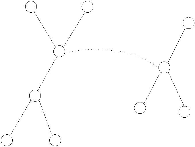
Exercise 2. For any undirected graph there is a pair of nodes s, t and an s-t minimum cut consisting
of a singleton node (either s or t). Such a pair is called a pendant pair.
Exercise 3. Let G be a graph such that deg(v) ≥ k for all v ∈ V . Show that there is some pair s, t
such that α (s, t) ≥ k.
G
Notice that the proof of the correctness of the algorithm relied only on the key lemma which in
turn used only the symmetry and submodularity of the cut function. One can directly extend the
proof to show the following theorem.
Theorem 5. Let V be a ground set, and let f : 2V → R+ be a symmetric submodular function.
Given s, t in V , define the minimum cut between s and t as
αf (s, t) =
min
W⊆V,|W∩{s,t}|=1
f(W)
Then, there is a Gomory-Hu tree that represents α . That is, there is a tree T = (V, E ) and a
f
T
capacity function c : ET → R+ such that α (s, t) = α (s, t) for all s, t in V , and moreover, the
f
T
minimum cut in T induces a minimum cut according to f for each s, t.
Exercise 4. Let G = (V, ξ) be a hypergraph. That is, each hyper-edge S ∈ ξ is a subset of V . Define
f : 2
V → R+ as
f W
(
δ W
) = | ( )|, where
S
∈
ξ
is in ( ) iff
δ W
S
∩
W
and
S
\
W
are non-empty.
Show that f is a symmetric, submodular function.
References
[
1] R. E. Gomory, T. C. Hu. Multi-terminal network flows. Journal of the Society for Industrial
and Applied Mathematics, vol. 9, 1961.
[
[
2] D. R. Karger. Minimum cuts in near-linear time. Journal of the ACM, vol. 47, 2000.
3] A. Schrijver. Combinatorial Optimization. Springer-Verlag Berlin Heidelberg, 2003. Chapter
1
5.4.
[
4] V. Vazirani. Approximation Algorithms. Springer, 2004.
CS 598CSC: Combinatorial Optimization
Instructor: Chandra Chekuri
Lecture date: Feb 9, 2010
Scribe: Matthew Yancey
1
Matchings in Non-Bipartite Graphs
We discuss matching in general undirected graphs. Given a graph G, ν(G) denotes the size of the
largest matching in G. We follow [1] (Chapter 24).
1
.1 Tutte-Berge Formula for ν(G)
Tutte (1947) proved the following basic result on perfect matchings.
Theorem 1 (Tutte) A graph G = (V, E) has a prefect matching iff G − U has at most |U| odd
components for each U ⊆ V .
Berge (1958) generalized Tutte’s theorem to obtain a min-max formula for ν(G) which is now
called the Tutte-Berge formula.
Theorem 2 (Tutte-Berge Formula) For any graph G = (V, E),
|
V |
o(G − U) − |U|
ν(G) =
− max
2
2
U⊆V
where o(G − U) is the number of components of G − U with an odd number of vertices.
Proof: We have already seen the easy direction that for any U, ν(G) ≤ |V | − o(G−U)−|U| by noticing
2
2
that o(G − U) − |U| is the number of nodes from the odd components in G − U that must remain
unmatched.
Therefore, it is sufficient to show that ν(G) = |V | − max
o(G−U)−|U|. Any reference to
U⊆V
2
2
left-hand side (LHS) or right-hand side (RHS) will be in reference to this inequality. Proof via
induction on |V |. Base case of |V | = 0 is trivial.
Case 1: There exists v ∈ V such that v is in every maximum matching. Let G0 =
(V 0, E0) = G − v, then ν(G0) = ν(G) − 1 and by induction, there is U0 ⊆ V 0 such that the RHS of
the formula is equal to ν(G0) = ν(G) − 1. It is easy to verify that U = U0 ∪ {v} satisfies equality
in the formula for G.
Case 2: For every v ∈ G, there is a maximum matching that misses it. By Claim 3
below, ν(G) = |V |−1 and that there is an odd number of vertices in the entire graph. If we take
2
U = ∅, then the theorem holds.
2
Claim 3 Let G = (V, E) be a graph such that for each v ∈ V there is a maximum matching in G
that misses v. Then, ν(G) = |V |−1. In particular, |V | is odd.
2
Proof: G is necessarily connected. By way of contradiction, assume there exists two vertices u = v
and a maximum matching M that avoids them. Among all such choices, choose M, u, v such that
dist(u, v) is minimized. If dist(u, v) = 1 then M can be grown by adding uv to it. Therefore there








exists a vertex t, u = t = v, such that t is on a shortest path from u to v. Also, by minimality of
distance between u and v we know that t ∈ M.
By the assumption, there is at least one maximum matching that misses t. We are going to
choose a maximum matching N that maximizes N ∩ M while missing t. N must cover u, or else
N, u, t would have been a better choice above. Similarly, N covers v. Now |M| = |N| and we have
found one vertex t ∈ M − N and two u, v ∈ N − M, so there must be another vertex x ∈ M − N
that is different from all of the above. Let xy ∈ M. N is maximal, so xy can’t be added to it.
Thus, we must have that y ∈ N and that means y = t. Let yz ∈ N. Then we have that z ∈ N −M
because xy ∈ M and z = x.
Figure 1: Green vertices are in M. Blue vertices are in N.
Consider the matching N0 = N − yz + xy. We have that |N0| = |N| and N0 avoids t and
0
. This is a contradiction.
|
N ∩ M| > |N ∩ M|
2
2
Algorithm for Maximum Cardinality Matching
We now describe a polynomial time algorithm for finding a maximum cardinality matching in a
graph, due to Edmonds. Faster algorithms are now known but the fundamental insight is easier to
see in the original algorithm. Given a matching M in a graph G, we say that a node v is M-exposed
if it is not covered by an edge of M.
Definition 4 A path P in G is M-alternating if every other edge is in M. It can have odd or even
length. A path P is M-augmenting if it is M-alternating and both ends are M-exposed.
Lemma 5 M is a maximum matching in G if and only if there is no M-augmenting path.
Proof: If there is an M-augmenting path, then we could easily use it to grow M and it would not
be a maximum matching.
In the other direction, assume that M is a matching that is not maximum by way of contradic-
tion. Then there is a maximum matching N, and |N| > |M|. Let H be a subgraph of G induced
by the edge set M∆N = (M − N) ∪ (N − M) (the symmetric difference). Note that the maximum
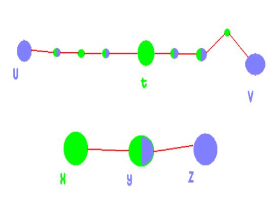
degree of a node in H is at most 2 since a node can be incident to at most one edge from N − M
and one edge from M − N. Therefore, H is a disjoint collection of paths and cycles. Furthermore,
all paths are M-alternating (and N-alternating too). All cycles must be of even length, since they
alternate edges from M and N too. At least one of the paths must have more N edges than M
edges because |N| > |M| and we deleted the same number of edges from N as M. That path is an
M-augmenting path.
2
The above lemma suggests a greedy algorithm for finding a maximum matching in a graph
G. Start with a (possibly empty) matching and iteratively augment it by finding an augmenting
path, if one exists. Thus the heart of the matter is to find an efficient algorithm that given G and
matching M, either finds an M-augmenting path or reports that there is none.
Bipartite Graphs: We quickly sketch why the problem of finding M-augmenting paths is rela-
tively easy in bipartite graphs. Let G = (V, E) with A, B forming the vertex bipartition. Let M
be a matching in G. Let X be the M-exposed vertices in A and let Y be the M-exposed vertices
in B. Obtain a directed graph D = (V, E0) by orienting the edges of G as follows: orient edges in
M from B to A and orient edges in E \ M from A to B. The following claim is easy to prove.
Claim 6 There is an M-augmenting path in G if and only if there is an X-Y path in the directed
graph D described above.
Non-Bipartite Graphs: In general graphs it is not straight forward to find an M-augmenting
path. As we will see, odd cycles form a barrier and Edmonds discovered the idea of shrinking
them in order to recursively find a path. The first observation is that one can efficiently find an
alternating walk.
Definition 7 A walk in a graph G = (V, E) is a finite sequence of vertices v , v , v , . . . , v such
0
1
2
t
that vivi+1 ∈ E, 0 ≤ i ≤ t − 1. The length of the walk is t.
Note that edges and nodes can be repeated on a walk.
Definition 8 A walk v , v , v , . . . , v is M-alternating walk if for each 1 ≤ i ≤ t − 1, exactly one
0
1
2
t
of v v and v v is in M.
i−1
i
i
i+1
Lemma 9 Given a graph G = (V, E), a matching M, and M-exposed nodes X, there is an O(|V |+
|
E|) time algorithm that either finds a shortest M-alternating X-X walk of positive length or reports
that there is no such walk.
Proof Sketch. Define a directed graph D = (V, A) where A = {(u, v) : ∃x ∈ V, ux ∈ E, xv ∈ M}.
Then a X-X M-alternating walk corresponds to a X-N(X) directed path in D where N(X) is the
set of neighbors of X in G (we can assume there is no edge between two nodes in X for otherwise
that would be a shortest walk). Alternatively, we can create a bipartite graph with D = (V ∪V 0, A)
where V 0 is a copy of V and A = {(u, v0) | uv ∈ E \ M} ∪ {(u0, v) | uv ∈ M} and find a shortest
X-X0
directed path in
D
where 0 is the copy of
X
X
in 0.
V
2
What is the structure of an X-X M-alternating walk? Clearly, one possibility is that it is
actually a path in which case it will be an M-augmenting path. However, there can be alternating
walks that are not paths as shown by the figure below.
One notices that if an X-X M-alternating walk has an even cycle, one can remove it to obtain
a shorter alternating walk. Thus, the main feature of an alternating walk when it is not a path is
the presence of an odd cycle called a blossom by Edmonds.
Definition 10 An M-flower is an M-alternating walk v , v , . . . , v such that v ∈ X, t is odd and
0
1
t
o
v = v for some even i < t. In other words, it consists of an even length v , . . . , v M-alternating
t
i
0
i
path (called the stem) attached to an odd cycle vi, vi+1, . . . , v = v called the M-blossom. The node
t
i
vi is the base of the stem and is M-exposed if i = 0, otherwise it is M-covered.
Figure 2: A M-flower. The green edges are in the matching
Lemma 11 A shortest positive length X-X M-alternating walk is either an M-augmenting path
or contains an M-flower as a prefix.
Proof: Let v , v , . . . , v be a shortest X-X M-alternating walk of positive length. If the walk is
0
1
t
a path then it is M-augmenting. Otherwise let i be the smallest index such that v = v for some
i
j
j > i and choose j to be smallest index such that v = v . If v , . . . , v is an even length cycle we
i
j
i
j
can eliminated it from the walk and obtain a shorter alternating walk. Otherwise, v , . . . , v , . . . , v
0
i
j
is the desired M-flower with vi as the base of the stem.
2
Given a M-flower and its blossom B (we think of B as both a set of vertices and an odd cycle),
we obtain a graph G/B by shrinking B to a single vertex b and eliminating loops and parallel edges.
It is useful to identify b with the base of the stem. We obtain a matching M/B in G/B which
consists of eliminating the edges of M with both end points in B. We note that b is M/B-exposed
iff b is M-exposed.
Theorem 12 M is a maximum matching in G if and only if M/B is a maximum matching in
G/B.
Proof: The next two lemmas cover both directions.
2
To simplify the proof we do the following. Let P = v , . . . , v be the stem of the M-flower.
0
i
Note that P is an even length M-alternating path and if v = v then v is M-exposed and v is
0
i
0
i
M-covered. Consider the matching M0
=
∆ ( ), that is by switching the matching edges in
M E P
P into non-matching edges and vice-versa. Note that |M |
0
=
|M|
and hence
M
is a maximum
matching in G iff M0 is a maximum matching. Now, the blossom B = v , . . . , v = v is also a
i
t
i
M0-flower but with a degenerate stem and hence the base is
M0-exposed. For the proofs to follow
we will assume that M = M0 and therefore b is an exposed node in G/B. In particular we will
assume that B = v , v , . . . , v = v with t odd.
0
1
t
0
Proposition 13 For each v in B there is an even-length M-alternating path Q from v to v .
i
i
0
i
Proof: If i is even then v , v , . . . , v is the desired path, else if i is odd, v = v , v , . . . , vi is the
0
1
i
0
t
t−1
desired path. That is, we walk along the odd cycle one direction or the other to get an even length
path.
2
Lemma 14 If there is an M/B augmenting path P in G/B then there is an M-augmenting path
in . Moreover, 0 can be found from in ( ) time.
0
P
G
P
P
O m
Proof:
Case 1: P does not contain b. Set P0 = P.
Case 2: P contains b. b is an exposed node, so it must be an endpoint of P. Without loss of
generality, assume b is the first node in P. Then P starts with an edge bu ∈ M/B and the edge bu
corresponds to an edge v u in G where v ∈ B. Obtain path P0 by concatenating the even length
i
i
M-alternating path Q from v to v from Proposition 13 with the path P in which b is replaced
i
0
i
by vi; it is easy to verify that is an M-augmenting path in G.
2
Lemma 15 If P is an M-augmenting path in G, then there exists an M/B augmenting path in
G/B.
Proof: Let P = u , u , . . . , u be an M-augmenting path in G. If P ∩ B = ∅ then P is an
0
1
s
M/B augmenting path in G/B and we are done. Assume u = v - if this is not true, flip the
0
0
path backwards. Let u be the first vertex in P that is in B. Then u , u , . . . , u , b is an M/B
j
0
1
j−1
augmenting path in G/B. Two cases to verify when u = v and when u = v for i = 0, both are
j
0
j
i
easy.
2
Remark 16 The proof of Lemma 14 is easy when b is not M-exposed. Lemma 15 is not straight
forward if b is not M-exposed.
From the above lemmas we have the following.
Lemma 17 There is an O(nm) time algorithm that given a graph G and a matching M, either
finds an M-augmenting path or reports that there is none. Here m = |E| and n = |V |.
Proof: The algorithm is as follows. Let X be the M-exposed nodes. It first computes a shortest
X-X M-alternating walk P in O(m) time — see Lemma 9. If there is no such walk then clearly
M is maximum and there is no M-augmenting path. If P is an M-augmenting path we are done.
Otherwise there is an M-flower in P and a blossom B. The algorithm shrinks B and obtains
G/B and M/B which can be done in O(m) time. It then calls itself recursively to find an M/B-
augmenting path or find out that M/B is a maximum matching in G/B. In the latter case, M is
a maximum matching in G. In the former case the M/B augmenting path can be extended to an
M-augmenting path in O(m) time as shown in Lemma 14. Since G/B has at least two nodes less
than G, it follows that his recursive algorithm takes at most O(nm) time.
2
By iteratively using the augmenting algorithm from the above lemma at most n/2 times we
obtain the following result.
Theorem 18 There is an O(n2m) time algorithm to find a maximum cardinality matching in a
graph with n nodes and m edges.
√
The fastest known algorithm for this problem has a running time of O(m n) and is due to
Micali and Vazirani with an involved formal proof appearing in [3]; an exposition of this algorithm
can be found in [2].
References
[
[
1] A. Schrijver. Combinatorial Optimization. Springer-Verlag Berlin Heidelberg, 2003
2] P. Peterson and M. Loui. The General Maximum Matching Algorithm of Micali and Vazirani.
Algorithmica, 3:511-533, 1998.
[
3] V. Vazirani. A Theory of Alternating Paths and Blossoms for Proving Correctness of the
p
O(|E| |V |) General Graph Maximum Matching Algorithm. Combinatorica, 14(1):71–109,
1
994.


CS 598CSC: Combinatorial Optimization
Instructor: Chandra Chekuri
Lecture date: 11 February, 2010
Scribe: Chandra Chekuri
1
Edmonds-Gallai Decomposition and Factor-Critical Graphs
This material is based on [1], and also borrows from [2] (Chapter 24).
Recall the Tutte-Berge formula for the size of a maximum matching in graph G.
Theorem 1 (Tutte-Berge) Given a graph G, the size of a maximum cardinality matching in G,
denoted by ν(G), is given by:
1
ν(G) = min (|V | + |U| − o(G − U))
2
U⊆V
where o(G − U) is the number of connected components in G[V \ U] with odd cardinality.
We call a set U that achieves the minimum on the right hand side of the Tutte-Berge formula,
a Tutte-Berge witness set. Such a set U gives some information on the set of maximum matchings
in G. In particular we have the following.
•
•
All nodes in U are covered in every maximum matching of G.
If K is the vertex set of a component of G−U, then every maximum matching in G covers at
least bK/2c nodes in K. In particular, every node in an even component is covered by every
maximum matching.
A graph can have different Tutte-Berge witness sets as the example in Fig 1 shows. Clearly
U = {v} is more useful than U = ∅.
v
Figure 1: Graph G above has 13 nodes, and ν(G) = 6. U = ∅ and U = {v} are both Tutte-Berge
witness sets.
A natural question is whether each graph has a canonical Tutte-Berge witness set that gives
us as much information as possible. The content of the Edmonds-Gallai decomposition is to give


a description of such a canonical witness set. Before we give the theorem, we digress to describe
some other settings with canonical witness sets. The reader can skip the next paragraph.
Let D = (V, A) be a directed graph and s, t ∈ V . It is easy to see that s has no directed path to
t iff there is a set X ⊆ V such that s ∈ X, t ∈ X and δ
+
( ) = ∅, that is no arcs leave . Among
X
X
all such sets X, the set X∗ defined as the set of all nodes reachable from s, is a canonical set. It
is a simultaneous witness for all nodes that are not reachable from s. Moreover, most algorithms
for checking reachability of t from s would output X∗. Similarly, consider the s-t maximum flow
problem in a capacitated directed graph D. By the maxflow-mincut theorem, the maximum flow
value F is equal to the capacity of a minimum capacity cut δ(X) that separates s from t. Again,
there could be multiple minimum cuts. One can show that if δ(X) and δ(Y ) are s-t minimum cuts
(here X and Y contain s and do not contain t) then δ(X ∩ Y ) and δ(X ∪ Y ) are also minimum
cuts (follows from submodularity of the cut function). From this, it follows that there exists a
unique minimal minimum cut δ(X∗) and a unique maximal minimum cut δ(Y ∗). We note that
X∗
is precisely the set of vertices reachable from in the residual graph of any maximum flow;
s
similarly V \ Y ∗ is the set of nodes that can reach t in the residual graph of any maximum flow.
Factor-Critical Graphs: If U is a non-empty Tutte-Berge witness set for a graph G, then it
follows that there are nodes in G that are covered in every maximum matching.
Definition 2 A graph G = (V, E) is factor-critical if G has no perfect matching but for each v ∈ V ,
G − v has a perfect matching.
Factor-critical graphs are connected and have an odd number of vertices. Simple examples
include odd cycles and the complete graph on an odd number of vertices.
Theorem 3 A graph G is factor-critical if and only if for each node v there is a maximum matching
that misses v.
Proof: If G is factor-critical then G − v has a perfect matching and hence a maximum matching
in G. We saw the converse direction in the proof of the Tutte-Berge formula — it was shown that
if each node v is missed by some maximum matching then G has a matching of size (|V | − 1)/2. 2
If G is factor-critical then U = ∅ is the unique Tutte-Berge witness set for G for otherwise there
would be a node that is in every maximum matching. In fact the converse is also true, but is not
obvious. It is an easy consequence of the Edmonds-Gallai decomposition to be seen shortly. We
give a useful fact about factor-critical graphs.
Proposition 4 Let C be an odd cycle in G. If the graph G/C, obtained by shrinking C into a
single vertex, is factor-critical then G is factor-critical.
Proof Sketch. Let c denote the vertex in G/C in place of the shrunken cycle C. Let v be an
arbitrary node in V (G). We need to show that G − v has a perfect matching.
If v ∈ C then G/C − v has a perfect matching M that matches c, say via edge cu. When we
unshrink c into C, let w be the vertex in C that corresponds to the edge cu. We can extend M a
perfect matching in G − v by adding edges in the even length path C − w to cover all the nodes in
C − w.
If v ∈ C, consider a perfect matching M in G/C − c. It is again easy to extend M to a perfect
matching in G − v by considering C − v.
2
We will see later a structural characterization of factor-critical graphs via ear decompositions.
1
.1 Edmonds-Gallai Decomposition
Theorem 5 (Edmonds-Gallai) Given a graph G = (V, E), let
D(G) := {v ∈ V | there exists a maximum matching that misses v}
A(G) := {v ∈ V | v is a neighbor of D(G) but v ∈ D(G)}
C(G) := V \ (D(G) ∪ A(G)).
Then, the following hold.
1
2
3
4
. The set U = A(G) is a Tutte-Berge witness set for G.
. C(G) is the union of the even components of G − A(G).
. D(G) is the union of the odd components of G − A(G).
. Each component in G − A(G) is factor-critical.
C(G)
A(G)
D(G)
Figure 2: Edmonds-Gallai Decomposition
Corollary 6 A graph G is factor-critical if and only if U = ∅ is the unique Tutte-Berge witness
set for G.
We prove the theorem in the rest of this section. We make use of the properties, and proof
of correctness, of Edmonds algorithm for maximum cardinality matching that we discussed in the
previous lecture.
Let M be any maximum matching in G and let X be the M-exposed nodes. We define three
sets of nodes with respect to M and X.
Even(G, M) := {v ∈ V | there is an even length M-alternating X-v path}
Odd(G, M) := {v ∈ V | there is an M-alternating X-v path} \ Even
Free(G, M) := {v ∈ V | there is no M-alternating X-v path}
Note that v ∈ Odd(G, M) implies that there is an odd length M-alternating X-v path but no
even length path. A node v ∈ Even(G, M) may have both an even and odd length path; also
X ⊆ Even(G, M).
Lemma 7 For any maximum matching M in G we have (i) Even(G, M) = D(G) (ii) Odd(G, M) =
A(G) and (iii) Free(G, M) = C(G).
Proof: We prove the claims in order. If v ∈ Even(G, M), let P be an even length M-alternating
path from some x ∈ X to v. Then, M∆E(P) is another maximum matching in which v is exposed;
hence, v ∈ D(G). Conversely, if v ∈ D(G) there is a maximum matching M that misses v. Then
v
M∆M gives an even length X-v M-alternating path implying that v ∈ Even(G, M). Therefore,
v
Even(G, M) = D(G).
If v ∈ Odd(G, M), let P be an X-v M-alternating path. Since v ∈ Even(G, M), P is of odd
length and its last edge is uv where u ∈ Even(G, M). Therefore v is a neighbor of Even(G, M) =
D(G) and v ∈ D(G) and hence v ∈ A(G). Conversely, suppose v ∈ A(G) and let uv ∈ E where
u ∈ D(G) = Even(G, M). There is an M-alternating X-u path P of even length which ends in
an edge wu ∈ M. If v ∈ V (P) then clearly there is an X-v alternating path. Otherwise, P + uv
is an X-v alternating path (wu ∈ M, hence uv ∈ M unless w = v but then v ∈ V (P)). Therefore
v ∈ Odd(G, M) since v ∈ D(G) = Even(G, M).
Finally, C(G) = V \ (D(G) ∪ A(G)) and hence Free(G, M) = C(G).
2
Lemma 8 Let M be any maximum matching in G, then each node in A(G) ∪ C(G) is covered by
M and moreover every node v ∈ A(G) is matched to some node in D(G).
Proof: From Lemma 7, X ⊆ D(G) where X is the set of M-exposed nodes. Hence each node in
A(G) ∪ C(G) is covered by M.
Suppose u ∈ A(G) and uv ∈ M. Since u ∈ Odd(G, M), there is an odd length X-v alternating
path P which ends in an edge wu ∈ M. If v is not in P then P + uv is an M-alternating X-v path
and hence v ∈ Even(G, M) = D(G). If v is in P, let Q be the prefix of P till v, then Q + vu is an
even length M-alternating X-u path which contradicts the fact that u ∈ A(G).
Corollary 9 Each component in G[C(G)] is even and |M ∩ C(G)| = |C(G)|/2.
2
Proof: All nodes in C(G) are covered by M. Since A(G) separates D(G) from C(G), and A(G)
is matched only to D(G) (by the above lemma), nodes in C(G) are matched internally and hence
the corollary follows.
2
The main technical lemma is the following.
Lemma 10 Let M be a maximum matching in G and X be the M-exposed nodes. Each component
H of G[D(G)] satisfies the following properties:
1
2
. Either |V (H) ∩ X| = 1 and |M ∩ δ (V (H))| = 0, or |M ∩ δ (V (H))| = 1.
. H is factor-critical.
G
G
Assuming the above lemma, we finish the proof of the theorem. Since each component of
G[D(G)] is factor-critical, it is necessarily odd. Hence, from Corollary 9 and Lemma 10, we have
that G[C(G)] contains all the even components of G − A(G) and G[D(G)] contains all the odd
components of G − A(G). We only need to show that A(G) is a Tutte-Berge witness. To see
this, consider any maximum matching M and the M-exposed nodes X. We need to show |M| =
1
2
(
+
( )
(
( ))). Since
= 1(
), this is equivalent to showing that
|
V | |A G | − o G − A G
|M|
|V | − |X|
2
|
X| + |A(G)| = o(G − A(G)). From Lemma 8, M matches each node in A(G) to a node in D(G).
From Lemma 10, each odd component in G[D(G)] either has a node in X and no M-edge to A(G) or
has exactly one M-edge to A(G). Hence |X| + |A(G)| = o(G − A(G)) since all the odd components
in G − A(G) are in G[D(G)].
We need the following proposition before the proof of Lemma 10.
Proposition 11 Let M be a maximum matching in G. If there is an edge uv ∈ G such that
u, v ∈ Even(G, M), then there is an M-flower in G.
Proof Sketch. Let P and Q be even length M-alternating paths from X to u and v, respectively.
If uv = M then P + uv + Q is an X-X alternating walk of odd length; since M is maximum, this
walk has an M-flower. If uv ∈ M, then uv is the last edge of both P and Q and in this case
P − uv + Q is again an X-X alternating walk of odd length.
2
Proof of Lemma 10. We proceed by induction on |V |. Let M be a maximum matching in G and
X be the M-exposed nodes. First, suppose D(G) is a stable set (independent set). In this case,
each component in G[D(G)] is a singleton node and the lemma is trivially true.
If G[D(G)] is not a stable set, by Proposition 11, there is an M-flower in G. Let B the M-
blossom with the node b as the base of the stem. Recall that b has an even length M-alternating
path from some node x ∈ X; by going around the odd cycle according to required parity, it can be
seen that B ⊆ Even(G, M) = D(G). Let G0 = G/B be the graph obtained by shrinking B. We
identify the shrunken node with b. Recall from the proof of correctness of Edmonds algorithm that
M0 M/B
=
is a maximum matching in G0. Moreover, the set of M0-exposed nodes in G0 is also
X
(note that we identified the shrunken node with b, the base of the stem, which belong to X if the
stem consists only of b). We claim the following with an informal proof.
Claim 12 D(G0) = (D(G) \ B) ∪ {b}, and A(G0) = A(G) and C(G0) = C(G).
Proof Sketch. We observed that X is the set of exposed nodes for both M and M0. We claim
that v ∈ Even(G0, M0) implies v ∈ Even(G, M). Let P be an even length X-v M0-alternating
path in G0. If it does not contain b then it is also an X-v even length M-alternating path in G. If P
contains b, then one can obtain an even length X-v M-alternating path Q in G by expanding b into
B and using the odd cycle B according to the desired parity. Conversely, let v ∈ Even(G, M) \ B
and let P be an X-v M-alternating path of even length in G. One can obtain an even length X-v
M0-alternating path in
Q
G0 as follows. If
P
does not intersect then
B
Q
=
P
suffices. Otherwise,
we consider the first and last nodes of P ∩B and shortcut P between them using the necessary parity
by using the odd cycle B and the matching edges in there. Therefore, D(G0) = (D(G) \ B) ∪ {b}
and the other claims follow.
2
By induction, the components of G0 − A(G0) satisfy the desired properties. Except for the
component H that contains b, every other such component is also a component in G − A(G).
b
Therefore, it is not hard to see that it is sufficient to verify the statement for the component H in
G − A(G) that contains B which corresponds to H in G − A G
0
(
0) that contains . We note that
b
b


X is also the set of M0
matched by M except possibly for b), the first desired property is easily verified.
-exposed nodes in
( )
G0 and since δG H ∩ M
=
δ
(
Hb ∩ M0 (B
)
is internally
G0
It remains to verify that H is factor-critical. By induction, H is factor-critical. Since H is
b
b
obtained by shrinking an odd cycle in H, Proposition 4 show that H is factor-critical.
2
Algorithmic aspect: Given G, its Edmonds-Gallai decomposition can be efficiently computed
by noting that one only needs to determine D(G). A node v is in D(G) iff ν(G) = ν(G − v) and
hence one can use the maximum matching algorithm to determine this. However, as the above proof
shows, one can compute D(G) in the same time it takes to find ν(G) via the algorithm of Edmonds,
which has an O(n3) implementation. The proof also shows that given a maximum matching M,
D(G) can be obtained in O(n2
) time.
1
.2 Ear Decompositions and Factor-Critical Graphs
A graph H is obtained by adding an ear to G if H is obtained by adding to G a path P that
connects two not-necessarily distinct nodes u, v in G. The path P is called an ear. P is a proper
ear if u, v are distinct. An ear is an odd (even) ear if the length of P is odd (even). A sequence of
graph G , G , . . . , G = G is an ear decomposition for G starting with G if for each 1 ≤ i ≤ k, G
0
1
k
0
i
is obtained from G
by adding an ear. One defines, similarly, proper ear decomposition and odd
i−1
ear decomposition by restricting the ears to be proper and odd respectively.
proper odd ear
proper even ear
not a proper ear
Figure 3: Variety of ears.
The following theorems are well-known and standard in graph theory.
Theorem 13 (Robbins, 1939) A graph G is 2-edge-connected if and only if it has an ear-decomposition
starting with a cycle.
Theorem 14 (Whitney, 1932) A graph G is 2-node-connected if and only if it has a proper
ear-decomposition starting with a cycle.
Factor-critical graphs have the following characterization.
Theorem 15 (Lov´asz, 1972) A graph G is factor-critical if and only if it has an odd ear decom-
position starting with a single vertex.
Proof: If G has an odd ear decomposition it is factor-critical by inductively using Proposition 4
and noting that an odd cycle is factor-critical for the base case.
We now prove the converse. G is necessarily connected. Let v be an arbitrary vertex and let
M be a perfect matching in G − v. We iteratively build the ear decomposition starting with the
v
empty graph v. At each step we maintain a (edge-induced) subgraph H of G such that H has
an odd ear decomposition and no edge uv ∈ M crosses H (that is, |V (H) ∩ {u, v}| = 1). The
v
process stops when E(H) = E(G). Suppose E(H) = E(G), then since G is connected, there is
some edge ab ∈ E(G) such that a ∈ V (H) and b = V (H). By the invariant, ab ∈ M . Let M
v
b
be a perfect matching in G that misses b. Then M ∆M contains an even length M -alternating
b
v
v
path Q := u = b, u , . . . , u = v starting at b and ending at v. Let j be the smallest index such
0
1
t
that u ∈ V (H) (j exists since u = v belongs to V (H)); that is u is the first vertex in H that
j
t
j
the path Q hits starting from b. Then, by the invariant, u u ∈ M and hence j is even. The
j−1
j
v
path a, b = u , u , . . . , u is of odd length and is a valid ear to add to H while maintaining the
0
1
j
invariant. This enlarges H and hence we eventually reach G and the process generates an odd ear
decomposition.
2
One can extend the above proof to show that G is 2-node-connected and factor-critical iff it has
an proper odd ear decomposition starting from an odd cycle.
From Proposition 4 and Theorem 15, one obtains the following.
Corollary 16 G is factor-critical iff there is an odd cycle C in G such that G/C is factor-critical.
References
[
1] Lecture notes from Michel Goemans class on Combinatorial Optimization. http://math.mit.
edu/ goemans/18438/lec3.pdf, 2009.
[
2] A. Schrijver. Theory of Linear and Integer Programming (Paperback). Wiley, 1998.
CS 598CSC: Combinatorial Optimization
Instructor: Chandra Chekuri
Lecture date: 2/16/2009
Scribe: Vivek Srikumar
1
Perfect Matching and Matching Polytopes
Let G = (V, E) be a graph. For a set E0 ⊆ E, let χE0 denote the characteristic vector of E0 in R|E|.
We define two polytopes:
Pperfect matching(G) = convexhull({χM |M
is a perfect matching in
G}
)
Pmatching(G) = convexhull({χM |M
is a perfect in
G}
)
Edmonds gave a description of these polytopes. Recall that for bipartite graphs, Pperfect matching(G)
is given by
x (δ(v)) = 1 ∀v ∈ V
x(e) ≥ 0 ∀e ∈ E
and Pmatching(G) is given by
x (δ(v)) ≤ 1 ∀v ∈ V
x(e) ≥ 0 ∀e ∈ E
We saw an example of a non-bipartite graph, for which (1, 1, 1) is an optimum solution.
2
2
2
1
2
1
2
1
2
Hence, (perfect) matching polytope for non-bipartite graphs are not captured by the simple con-
straints that work for bipartite graphs.
Theorem 1 (Edmonds) Pperfect matching(G) is determined by the following set of inequalities.
x(e) ≥ 0;
e ∈ E
v ∈ V
x (δ(v)) = 1;
x (δ(U)) ≥ 1; U ⊆ V, |U| ≥ 3, |U| odd
Edmonds gave a proof via an algorithmic method. In particular, he gave a primal-dual algorithm
for the minimum cost perfect matching problem, which, as a by product showed that for any cost
vector c on the edges, there is a minimum cost perfect matching whose cost is equal the minimum
value of cx subjecto to the above set of inequalities. This implies that the polytope is integral. We
describe a short non-algorithmic proof that was given later [1] (Chapter 25).
Proof: Let Q(G) denote the polytope described by the inequalities in the theorem statement. It is
easy to verify that for each graph G, Pperfect matching(G) ⊆ Q(G). Suppose there is a graph G such



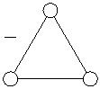


that Q(G) ⊆ P
(G). Among all such graphs, choose the one that minimizes |V |+|E|.
perfect matching
Let G be this graph. In particular, there is a basic feasible solution (vertex) x of Q(G) such that
x is not in Pperfect matching(G).
We claim that x(e) ∈ (0, 1); ∀e ∈ E. If x(e) = 0 for some e, then deleting e from G gives a
smaller counter example. If x(e) = 1 for some e, then deleting e and its end points from G gives a
smaller counter example.
We can assume that |V | is even, for otherwise Q(G) = ∅ (why?) and P
(G) = ∅
perfect matching
as well. Since 0 < x(e) < 1 for each e and x(δ(v) = 1 for all v, we can assume that deg(v) ≥
2
;
∀v ∈ V . Suppose |E| = 2|V |. Then deg(v) = 2; ∀v ∈ V and therefore, G is a collection
of vertex disjoint cycles. Then, either G has an odd cycle in its collection of cycles, in which
case, Q(G) = ∅ = Pperfect matching(G), or G is a collection of even cycles and, hence bipartite and
perfect matching
Q(G) = P
(G).
Thus |E| > 2|V |. Since x is a vertex of Q(G), there are |E| inequalities in the system that
are tight and determine x. Therefore, there is some odd set U ⊆ V such that x (δ(U)) = 1. Let
¯
¯
0
=
, where is shrunk to a node, say 0. Define 00 =
, where
=
is shrunk to a
G
G/U
U
u
G
G/U
U
V −U
node u00; see Figure 1. The vector x when restricted to G0 induces x0 ∈ Q(G0) and similarly x induces
¯
¯
U
U
U
U
e1
e1
e1
eh
u0
u00
eh
eh
(a) G
(b) G0
(c) G00
Figure 1:
, we have that
0
0
(
00). Since
G0 and G00 are smaller than
(
0) =
(G0)
perfect matching
x ∈ Q G
G
Q G
P
and Q(G00) = P
(G00). Hence, x0 can be written as a convex combination of perfect
perfect matching
matchings in G0 and x00 can be written as a convex combination of perfect matchings in G00. The
vector x is rational since we chose it as a vertex of Q(G), therefore, x0, x00 are also rational; hence,
P
0
= k1
k
M0 , where
0
0
0 are perfect matchings in
G0 and
∃
integer k such that x
0 = 1
χ
M , M , · · · , M
i
1
2
k
P
i=1
00
0
k
i=1
M00 , where
00
1
00 are perfect matchings in
G00. (Note that
is the same
x
χ
M , M , · · · , M
k
i
k
2
k
in both expressions.)
Let e , e , · · · , e be edges in δ(U). Since x0(δ(u0) = 1 and u0 is in every perfect matching,
1
2
h
we have that e is in exactly kx0(e ) = kx(e ) matchings of M0 , · · · , M0 . Similarly, e is in ex-
j
j
j
P
1
j
k
actly kx(e ) matchings of M00, · · · , M00. Note that
n
j=1
kx(e ) = k and moreover, exactly one of
j
1
M
j
k
e , · · · , e can be in M
0
i
and 00. We can, therefore, assume (by renumbering if necessary) that
M
0
i
1
h
i
and M00 share exactly one edge from e , · · · , e . Then, M = M0 ∪ M00 is a perfect matching in G.
i
P
1
h
i
i
i
Hence, x = 1
k
i=1
χM , which implies that x ∈ P
(G), contradicting our assumption.
i
perfect matching
k
2
Now, we use the above theorem to derive the following:


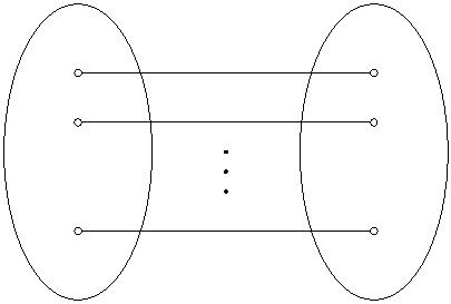
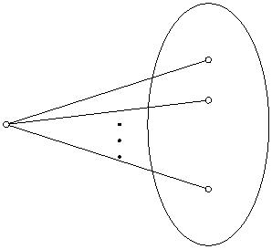
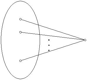


Theorem 2 Pmatching(G) is determined by
x(e) ≥ 0;
e ∈ E
v ∈ V
x (δ(v)) ≤ 1;
|
U| − 1
x (E[U]) ≤
; U ⊆ V, |U| odd
2
Here E[U] is the set of edges with both end points in U.
Proof: We can use a reduction of weighted matching to weighted perfect matching that is obtained
˜
˜ ˜
as follows: Given G = (V, E), create a copy G0 = (V 0, E0) of G. And let G be the graph (V , E)
defined as V = V ∪ V 0, E = E ∪ E0 ∪ {(v, v0) | v ∈ V }.
˜
˜
G0
, copy of
G
G
v
v0
The following claim is easy to prove.
˜
Claim 3 There is an injective mapping from the matchings in G to the perfect matchings in G.
Corollary 4 The maximum weight matching problem is poly-time equivalent to maximum weight
perfect matching problem.
We can use the above idea to establish the theorem. Let x be feasible for the system of
inequalities in the theorem. We show that x can be written a convex combination of matchings in
˜
G. It is clear that χ
M satisfies the inequalities for every matching . From , create as above
M
G
G
˜
and define a fractional solution x˜ : E → R+ as follows: first, we define x0 : E0 → R+ as the copy of
x on E. That is, x e
0
( 0) = ( ), where 0 is the copy of . Then,
x e
e
e
x(e); if e ∈ E
(e); if e ∈ E0
x˜ = x0
1
− x (δ(v)) ; if e = vv0
G0
G
0
.3
.1
0.3
0
.2
0.4
0.2
0
0.1

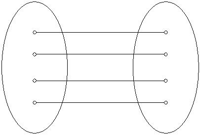
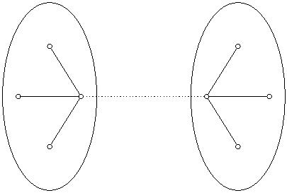
˜
Claim 5 x˜ belongs to Pperfect matching(G).
Assuming the claim, we see that x˜ can be written as a convex combination of perfect matchings
˜
˜
in G. Each perfect matching in G induces a matching in G and it is easy to verify that x can
therefore be written as a convex combination of matchings in G.
It only remains to verify the claim. From the previous theorem, it suffices to show that
ꢀ
ꢁ
˜
˜
x˜ δ(U) ≥ 1; ∀U ⊆ V , |U|odd
G0
G
U
X0
W
˜
Let U ⊆ V and |U| odd. Let W = U ∩ V and X0 = U ∩ V 0, where X0 is the copy of X ⊆ V .
First we consider the case that X0 = ∅ and |W| is odd. Then
ꢀ
ꢁ
ꢀ
ꢁ
˜
˜
x˜ δ(U) = x˜ δ(W)
ꢀ
ꢁ
X
˜
=
x˜ δ(v) − 2x˜ (E[W])
v∈W
=
≥
≥
|W| − 2x (E[W])
ꢂ
ꢃ
ꢁ
|
W| − 1
|W| − 2
2
1
ꢀ
ꢁ
ꢀ
ꢀ
ꢁ
˜
˜
˜
For the general case, we claim that x˜ δ(U) ≥ x˜ δ(W \ X) + x˜ δ(X0 \ W0) . Without loss of
ꢀ
ꢁ
ꢀ
ꢁ
˜
˜
generality, W \ X is odd. Then x˜ δ(U) ≥ x˜ δ(W \ X) ≥ 1 from above.
The claim can be verified as follows:
X0 \ W
0
X0
W
∩
X
W0 ∩ X0
W
W \ X
Notice that only edges between W and X0 are between W ∩X and X0∩W0. Let A = W ∩X, A0 =


W0 ∩ X0. Then
ꢀ
ꢁ
ꢀ
ꢁ
˜
˜
x˜ δ(U) = x˜ δ(W ∪ X
0)
ꢀ
ꢁ
ꢀ
ꢄ ꢄ
ꢁ
˜
˜
=
x˜ δ(W \ X) + x˜ δ(X0 \ W0) +
x (δ(A)) − 2x((δ (E[A, W \ X])) +
ꢄ
ꢅ
ꢅꢅ
0
(
0)
2
0
[
0
0
0]
x δ A − x δ E A , X \ W
The claim follows from the observation that x(δ(A)) ≥ x (E[A, W \ A]) + x (δ(E[A, X \ W]).
Corollary 6 Pperfect matching(G) is also determined by
2
x(e) ≥ 0;
e ∈ E
v ∈ V
x (δ(v)) = 1;
|
U| − 1
x (E[U]) ≤
; U ⊆ V, |U| odd
2
We note that although the system in the above corollary and the earlier theorem both determine
Pperfect matching(G), they are not identical.
2
Separation Oracle for Matching Polytope
The inequality systems that we saw for P
(G) and Pmatching(G) have an exponential
perfect matching
number of inequalities. Therefore, we cannot use them directly to solve the optimization problems
of interest, namely, the maximum weight matching problem or the minimum weight perfect match-
ing problem. To use the Ellipsoid method, we need a polynomial time separation oracle for the
polytopes. Edmonds gave efficient strongly polynomial time algorithms for optimizing over these
polytopes. From the equivalence of optimization and separation (via the ellipsoid method) implies
that there is a strongly polynomial time separation oracle. However, the oracle obtained via the
above approach is indirect and cumbersome. Padberg and Rao [1982] gave a simple and direct
separation oracle. We discuss this for the system
x(e) ≥ 0;
e ∈ E
v ∈ V
(1)
x (δ(v)) = 1;
x (δ(U)) ≥ 1; |U| odd, U ⊆ V
and it can be used with the reduction shown earlier for the matching polytope as well.
Theorem 7 There is a strongly polynomial time algorithm, that given G = (V, E) and x : E → R
determines if x satisfies (1) or outputs an inequality from (1) that is violated by x.
It is trivial to check the first two sets of inequalities. Therefore, we assume that x ≥ 0 and
x (δ(v)) = 1; ∀v ∈ V . We can also assume that |V | is even. Thus the question is whether there is
a set U ⊂ V, |U| odd, such that x (δ(U)) < 1. It is sufficient to give an algorithm for the minimum
odd-cut problem, which is the following: Given a capacitated graph G = (V, E), find a cut δ(U) of
minimum capacity among all sets U such that |U| is odd. We claim that the following is a correct
algorithm for the minimum odd-cut problem.




1
. Compute a Gomory-Hu tree T = (V, ET ) for G.
2
. Among the odd-cuts induced by the edges of T, output the one with the minimum capacity.
To see the correctness of the algorithm, let δ(U∗) be a minimum capacity odd cut in G. Then
) is a set of edges in . We claim that there is an edge has a
δT (U∗
ET
st ∈ δ U∗) such that T − st
(
T
component with an odd number of nodes. If this is true, then, by the prperties of the Gomory-Hu
tree, T −st induces an odd cut in G of capacity equal to α (s, t) (recall that α (s, t) is the capacity
G
G
of a minimum s-t cut in G). Since δ(U∗) separates s and t, the odd cut induced by T − st has no
larger capacity than δ(U∗). We leave it as an exercise to show that some edge in δ (U∗) induces
T
an odd-cut in T.
3
Edge Covers and Matchings
Given G = (V, E) an edge cover is the subset E0 ⊂ E such that each node is covered by some edge
in E0. This is the counterpart to vertex cover. Edge covers are closely related to matchings and
hence optimization problems related to them are tractable, unlike the vertex cover problem whose
minimization version is NP-Hard.
Theorem 8 (Gallai) Let ρ(G) be the cardinality of a maximum size edge cover in G. Then
ν(G) + ρ(G) = |V |
where ν(G) is the cardinality of a maximum matching in G.
Proof: Take any matching M in G. Then M covers 2|M| nodes, the end points of M. For
each such uncovered node, pick an arbitrary edge to cover it. This gives an edge cover of size
≤
|V | − 2|M| + |M| ≤ |V | − |M|. Hence ρ(G) ≤ |V | − ν(G).
We now show that ν(G) + ρ(G) ≥ |V |. Let E0 be any inclusion-wise minimal edge cover and let
M be an inclusion-wise maximal matching in E0
. If is not incident to an edge of
v
M
then since it
is covered by E0 there is an edge e ∈ E0 \M that covers v; since M is maximal the other end point
v
of e is covered by M. This implies that 2|M| + |E0 \ M| ≥ |V |, that is 2|M| + |E0| − |M| ≥ |V |
v
and hence |M| + |E0| ≥ |V |. If E0 is a minimum edge cover then |E0| = ρ(G) and |M| ≤ ν(G),
therefore, ν(G) + ρ(G) ≥ |V |.
2
The above proof gives an efficient algorithm to compute ρ(G) and also a minimum cardinality
edge cover via an algorithm for maximum cardinality matching. One can define the minimum
weight edge cover problem and show that this also has a polynomial time algorithm by reducing to
matching problems/ideas. The following set of inequalities determine the edge cover polytope (the
convex hull of the characterstic vectors of edge covers in G).
x (δ(V )) ≥
1
∀v ∈ V
U ⊆ V |U|odd
e ∈ E
x (E[U] ∪ δ(U)) ≥
|
U|+1
;
2
0
≤ x(e) ≤ 1;
Exercise 9 Prove that the polytope above is the edge cover polytope and obtain a polynomial time
separation oracle for it.

References
[
1] A. Schrijver. Combinatorial optimization: polyhedra and efficiency, Springer, 2003.
CS 598CSC: Combinatorial Optimization
Instructor: Nitish Korula
Lecture date: Feb 18, 2010
Scribe: Abner Guzm´an-Rivera
1
Maximum Weight Matching in Bipartite Graphs
In these notes we consider the following problem:
Definition 1 (Maximum Weight Bipartite Matching) Given a bipartite graph G = (V, E)
with bipartition (A, B) and weight function w : E → R find a matching of maximum weight where
P
the weight of matching M is given by w(M) =
w(e).
e∈M
Note that without loss of generality, we may assume that G is a complete weighted bipartite
graph (we may add edges of zero weight as necessary); we may also assume that G is balanced,
i.e. |A| = |B| = 1|V |, as we can add dummy vertices as necessary. Hence, some maximum weight
2
matching is a perfect matching. Furthermore, by negating the weights of the edges we can state
the problem as the following minimization problem:
Definition 2 (Minimum Weight Perfect Matching in Bipartite Graphs) Given a bipartite
graph G = (V, E) with bipartition (A, B) and weight function w : E → R ∪ {∞}, find a perfect
P
matching M minimizing w(M) =
w(e).
e∈M
We could also assume that no edge weights are negative as we may add a large enough constant
C to all weights, but this is not required by the algorithms below.
The following is an ILP formulation of the minimum weight perfect matching problem:
X
min
w(a, b)x(a, b) subject to:
(a,b)
X
x(a, b) = 1
∀a ∈ A
Xb
(1)
x(a, b) = 1
∀b ∈ B
a
x(a, b) ∈ {0, 1} ∀a ∈ A, b ∈ B
Definition 3 (Primal) This is the LP relaxation of the above ILP:
X
min
w(a, b)x(a, b) subject to:
(a,b)
X
x(a, b) = 1 ∀a ∈ A
Xb
(2)
x(a, b) = 1 ∀b ∈ B
x(a, b) ≥ 0 ∀a ∈ A, b ∈ B
a
Recall that we saw, in an earlier lecture, a proof of the following theorem by noting that the
constraint matrix of the polytope is totally unimodular.


Theorem 4 Any extreme point of the polytope defined by the constraints in (2) is integral.
We obtain a different proof of Theorem 4 via algorithms to find a minimum-weight perfect
matching. Our algorithms are primal-dual; we will construct a feasible solution to the dual of
LP (2) with value equal to the weight of the perfect matching output by the algorithm. By weak
duality, this implies that the matching is optimal. More precisely, our algorithms will always
maintain a feasible dual solution y, and will attempt to find a primal feasible solution (a perfect
matching M) that satisfies complementary slackness.
(Dual) The following LP is the dual for (2):
X
X
maximize
y(a) +
y(b) subject to:
(a∈A
b∈B
y(a) + y(b) ≤ w(a, b) ∀(a, b) ∈ E
(3)
Given a dual-feasible solution y, we say that an edge e = (a, b) is tight if y(a) + y(b) = w(a, b). Let
yˆ be dual-feasible, and let M be a perfect matching in G(V, E): Then,
X
X
w(M) =
w(a, b) ≥
yˆ(a) + yˆ(b)
(a,b)∈M
(a,b)∈M
X
X
=
=
yˆ(a) · (δ(a) ∩ M) +
yˆ(b) · (δ(b) ∩ M)
a∈A
b∈B
X
X
yˆ(a) +
yˆ(b)
a∈A
b∈B
where the first inequality follows from the feasibility of yˆ, and the final equality from the fact that
M is a perfect matching. That is, any feasible primal solution (a perfect matching M) has weight
at least as large as the value of any feasible dual solution. (One could conclude this immediately
from the principle of weak duality.) Note, though, that if M only uses edges which are tight under
yˆ, we have equality holding throughout, and so by weak duality, M must be optimal. That is, given
any dual feasible solution yˆ, if we can find a perfect matching M only using tight edges, M must
be optimal. (Recall that this is the principle of complementary slackness.)
Our primal-dual algorithms apply these observations as follows: We begin with an arbitrary
feasible dual solution y, and find a maximum-cardinality matching M that uses only tight edges.
If M is perfect, we are done; if not, we update our dual solution. This process continues until we
find an optimal solution.
We first give a simple algorithm (Algorithm 1 in the following page) exploiting these ideas to
prove Theorem 4. The existence of set S in line 6 is a consequence of Hall’s theorem. Observe that
the value of y increases at the end of every iteration. Also, the value of y remains feasible as tight
edges remain tight and it is easy to verify that by the choice of ꢀ the constraints for other edges
are not violated.
Claim 5 Algorithm 1 terminates if w is rational.
Proof: Suppose all weights in w are integral. Then at every iteration ꢀ is integral and furthermore
ꢀ
≥ 1. It follows that the number i of iterations is bounded by i ≤ max w(a, b) · |E|. If weights are
rational we may scale them appropriately so that all of them become integers.
2
Algorithm 1 MinWeightPerfectMatching(G = (V, E), w)
1
2
3
4
5
6
7
8
9
: y ← 0
0
set of tight edges
: E ←
: M ← max cardinality matching for graph G
0
= (V, E0)
: while M is not a perfect matching do
:
:
:
:
:
let G0
let S ⊆ A be such that |S| > |N(S)|
let ꢀ = min
{w(a, b) − y(a) − y(b)}
= (V, E0)
a∈S,b∈B\N(S)
∀a ∈ S y(a) = y(a) + ꢀ
∀b ∈ N(S) y(b) = y(b) − ꢀ
update E M
0
,
1
1
1
0:
1: end while
2: return M
Proof of Theorem 4. The incidence vector of a perfect matching computed by Algorithm 1 is an
extreme point of the polytope in (2). This vector is integral. Furthermore, by carefully choosing
the cost function one can make any extreme point be the unique optimum solution to the primal
linear program.
2
Note that Algorithm 1 does not necessarily terminate in strongly polynomial time; in the rest
of this section, we describe a more efficient algorithm for the minimum-weight bipartite matching
problem.
As before, Algorithm 2 always maintains a feasible dual y and attempts to find a close to
primal feasible solution (matching M) that satisfies complementary slackness. One key difference
from Algorithm 1 is that we now carefully use the maximum cardinality matching M as a guide in
constructing the updated dual solution y; this allows us to argue that we can augment M efficiently.
(In contrast, Algorithm 1 effectively “starts over” with a new matching M in each iteration.)
Algorithm 2 MinWeightPerfectMatchingPD(G = (V, E), w)
1
2
3
4
5
6
7
8
9
: ∀b ∈ B y(b) ← 0
: ∀a ∈ A y(a) ← min {w(a, b)}
b
0
set of tight edges
: E ←
: M ← max cardinality matching for graph G
0
= (V, E0)
: while M is not a perfect matching do
S
let Edir ← {e directed from A to B | e ∈ E , e ∈/ M}
0
0
:
:
:
:
{e directed from B to A | e ∈ E , e ∈ M}
let D = (V, Edir) {D is a directed graph}
let L ← {v | v is reachable in D from an unmatched vertex in A}
let ꢀ = min
1
1
1
1
1
1
0:
1:
2:
3:
{w(a, b) − y(a) − y(b)}
a∈A∩L,b∈B\L
∀a ∈ A ∩ L y(a) = y(a) + ꢀ
∀b ∈ B ∩ L y(b) = y(b) − ꢀ
update E M
0
,
4: end while
5: return M






Claim 6 At every iteration, C = (A \ L) ∪ (B ∩ L) is a vertex cover for graph G0 = (V, E0).
Moreover, |C| = |M|.
Proof: Assume C is not a vertex cover. Then there must be an edge e = (a, b) ∈ E0 with a ∈ A∩L
and b ∈ B \ L. If e is directed from a to b, then since a is reachable from an unmatched vertex in
A, so is b; this contradicts the fact that b ∈ B \ L. Therefore, e must be directed from b to a, and
hence e is in the matching M. As a itself is matched (using edge e) and a ∈ L, it must be reachable
from an unmatched vertex of A. But the only incoming edge to a is (b, a) (this is the unique edge
incident to a in the matching M), and hence b is reachable from this unmatched vertex of A; again,
this contradicts the fact that b ∈/ L. To show the second part of the proof we show that |C| ≤ |M|,
since the reverse inequality is true for any matching and any vertex cover. The proof follows from
the following observations:
1
. No vertex in A \ L is unmatched by the definition of L.
2
. No vertex in B ∩ L is unmatched since this would imply the existence of an augmenting path
(contradicting the maximality of M).
3
. There is no edge e = (a, b) ∈ M such that a ∈ A \ L and b ∈ B ∩ L. Otherwise, as this edge
would be directed from b to a, a would be in L.
These remarks imply that every vertex in C is matched and moreover the corresponding edges of
the matching are distinct. Hence |C| ≤ |M|, and so C is an optimum vertex cover for G0(V, E0). 2
At every iteration where the maximum cardinality matching M output is not perfect, the
algorithm will use information from the optimum vertex cover C to update the dual solution and
improve its value. By the proof of claim 6 there is no tight edge between a ∈ A ∩ L and b ∈ B \ L,
which implies ꢀ > 0; it is easy to check that the updated dual solution is feasible. Moreover, the
difference between the new dual solution and the old dual solution is:
|
V |
ꢀ
· (|A ∩ L| − |B ∩ L|) = ꢀ · (|A ∩ L| + |A \ L| − |A \ L| − |B ∩ L|) = ꢀ · (
− |C|),
2
but |C| = |M| < |V |, since M is not perfect, which implies the value of the dual solution strictly
2
increases. When the algorithm terminates, we obtain a perfect matching M and a dual feasible
solution which satisfy complementary slackness.
Claim 7 Algorithm (2) terminates in O(|V |2) iterations.
Proof: We first observe that after any iteration, all edges in M are still tight: The only edges (a, b)
that are tight at the beginning of an iteration but not at the end are those with a ∈ A ∩ L and
b ∈ B \ L; from observation 3 in the proof of Claim 6, there are no edges in M of this form. Thus,
after any iteration, the size of a maximum cardinality matching M in G0(V, E0) cannot decrease.
Say that an iteration is successful if the size of a maximum cardinality matching using the tight
edges E0 increases. Clearly, after at most |V |/2 successful iterations, we have a perfect matching,
and the algorithm terminates. We show that there are at most |B| = |V |/2 consecutive unsuccessful
iterations between any pair of successful iterations. Hence, the total number of iterations is at most
|
V | |V |, which is
(
).
·
O |V |2
2
2


To bound the number of consecutive unsuccessful iterations, we argue below that after an
unsuccessful iteration, |B ∩ L| increases. Assume for now that this is true: After at most |B|
unsuccessful iterations, we have B ∩ L = B. Once this occurs, every vertex of B (which must
include at least one unmatched vertex) is reachable from an unmatched vertex of A, and so we can
augment M to find a larger matching, which means that the current iteration is successful.
It remains only to prove that at every unsuccessful iteration, at least one more vertex in B
must become reachable from an exposed vertex in A (i.e. |B ∩ L| increases). First note that no
vertex of A or B becomes unreachable; the only way this could happen is if for some path P from
an unmatched vertex a ∈ A to vertex v ∈ L, an edge e ∈ P that was previously tight is no longer
tight. But the only edges that are no longer tight are between A \ L and B ∩ L, and by definition,
no such path P visits a vertex in A\L. To see that at least one new vertex of B becomes reachable,
note that some edge e = (a, b) with a ∈ A ∩ L and b ∈ B \ L now has become tight by our choice
of ꢀ. As the edge (a, b) is directed from a to b, b is now reachable.
2
It is not hard to see that each iteration takes only O(|V |2) time, and hence the overall running
time of the algorithm is O(|V |4). A more careful analysis would yield a tighter running time of
O(|V |
3
).
References
[
1] A. Schrijver. Combinatorial optimization: Polyhedra and Efficiency, Springer, 2003. Chapter
7.
1
[
2] Lecture notes from Michael Goemans class on Combinatorial Optimization. http://math.
mit.edu/ goemans/18433S09/matching-notes.pdf, 2009.
CS 598CSC: Combinatorial Optimization
Instructor: Chandra Chekuri
Lecture date: Fe b 23, 2010
Scribe: Rajhans Samdani
1
Min Cost Perfect Matching
In this lecture, we will describe a strongly polynomial time algorithm for the minimum cost perfect
matching problem in a general graph. Using a simple reduction discussed in lecture 9, one can
also obtain an algorithm for the maximum weight matching problem. We also note that when
discussing perfect matching, without loss of generality, we can assume that all weights/costs are
non-negative (why?).
The algorithm we describe is essentially due to Edmonds. The algorithm is primal-dual based
on the following LP formulation and its dual.
Primal:
X
min
w(e)x(e)
subject to:
e∈E
x(δ(v)) = 1 ∀v ∈ V
(1)
x(δ(U)) ≥ 1 ∀U ⊂ V, |U| ≥ 3, |U|odd
x(e) ≥ 0 ∀e ∈ E
Dual:
X
max
π(U)
subject to:
U⊆V,|U|≥3,|U|odd
X
π(U) = w(e) ∀e ∈ E
U⊆V,|U|≥3,|U|odd,δ(U)3e
π(U) ≥ 0
∀U ⊆ V, |U| ≥ 3, |U|odd
We note that non-negativity constraints on the dual variables are only for odd sets U that are not
singletons (because the equations for the singleton sets are equalities). In certain descriptions of
the algorithm and details, the dual variables for the singleton are distinguished from the odd sets
of size ≥ 3, however we don’t do that here.
Like other primal dual algorithms, we maintain a feasible dual solution π and an integral
infeasible primal solution x and iteratively reduce the infeasiblity of x. Here x corresponds to a
matching and we wish to drive it towards a maximum matching. In particular, we will also maintain
the primal complementary slackness, that is,
X
x(e) > 0 ⇒
π(U) = w(e)
U:e∈δ(U)
(a primal variable being positive implies the corresponding dual constraint is tight). Thus, at the
end, if we have a perfect matching in the primal, it is feasible and certifies its optimality.
The main question is how to update the dual and the primal. Also, we observe that the dual has
an exponential number of variables and hence any polynomial time algorithm can only maintain
an implicity representation of a subset of the variables.

1
.1 Notation
The algorithm maintains a laminar family of odd subsets of V denoted by Ω. Ω always includes the
singletons {v} , v ∈ V . It maintains the invariant that π(U) = 0 if U ∈/ Ω, hence Ω is the implicit
representation of the “interesting” dual variables. Note that |Ω| ≤ 2|V |.
Given G, Ω and π : Ω → R where π is dual feasible, we say an edge is π-tight (or tight when π
P
is implicit) if
π(U) = w(e).
U∈Ω:e∈δ(U)
Let E be the set of tight edges (with Ω, π implicit) and G be the graph induced by them.
π
π
We obtain a new graph G0 in which we contract each maximal set in Ω into a (pseudo) vertex. For
a node v ∈ G0, let S ∈ Ω be the set of nodes of G contracted to v.
v
For each U ∈ Ω, |U| ≥ 3, consider the graph G [U] and let H be the graph obtained from
π
U
G [U] by contracting each maximal proper subset S ⊂ U where S ∈ Ω. The algorithm also
π
maintains the invariant that HU has a Hamiltonian cycle B .
U
1
.2 Recap on Edmonds Gallai Decomposition
We restae the Edmonds Gallai decomposition and make some observations which help us in propos-
ing and analysing an algorithm for min cost perfect matching. We also use the notation from this
section in subsequent sections.
Theorem 1 (Edmonds-Gallai) Given a graph G = (V, E), let
D(G) := {v ∈ V | there exists a maximum matching that misses v}
A(G) := {v ∈ V | v is a neighbor of D(G) but v ∈ D(G)}
C(G) := V \ (D(G) ∪ A(G)).
Then, the following hold.
1
2
3
4
. The set U = A(G) is a Tutte-Berge witness set for G.
. C(G) is the union of the even components of G − A(G).
. D(G) is the union of the odd components of G − A(G).
. Each component in G − A(G) is factor-critical.
It is also easy to see the following remark.
Remark 2 Let M be a maximum matching in G. Then either there exist an M−blossom or D(G)
consists of singleton nodes.
1
.3 Algorithm
Following is the algorithm for min cost perfect matching using primal dual method.
Initialize: Ω = {{v}|v ∈ V }, π(U) = 0 ∀U with odd |U|, M = φ, and G0 = G .
π
while(M is not a perfect matching in G0) do
1
2
. X ← M−exposed nodes in G0.
. Find X − X, M−alternating walk P in G0.
3
4
5
. If P is an M−augmenting path then do
M ← M∆E(P)
continue.
. If P has an M−blossom B, then do shrinking as:
U = ∪v∈BS , Ω ← Ω ∪ U, π(U) = 0, G ← G /B, M ← M/B
0
0
v
continue.
. Else P is empty ⇒ M is a maximum matching in G0. Compute D(G0), A(G0), and C(G0) as in
Edmonds-Gallai decomposition. Let ꢀ be the largest value such that π(S ) = π(S ) + ꢀ, ∀v ∈
v
.
v
D(G0
π S
) and ( ) = (
π S − ꢀ, ∀v ∈ A G
)
(
0) maintains feasibility of in
π
G
v
v
If ꢀ is unbounded then G has no perfect matching; STOP.
If π(S ) = 0 for some v ∈ A(G0) and |S | ≥ 3, then deshrink as
v
v
•
•
•
Remove Sv from Ω.
Update Gπ and G0
.
Extend M by a perfect matching in BSv − {v}.
end while
Extend M in G0 to a perfect matching in Gπ and output it.
Example: Consider the execution of this algorithm on the following graph:
Figure 1: Original graph G
The execution is shown in figures 2 to 9. Red edges are the current edges in the matching; black
edges are tight.
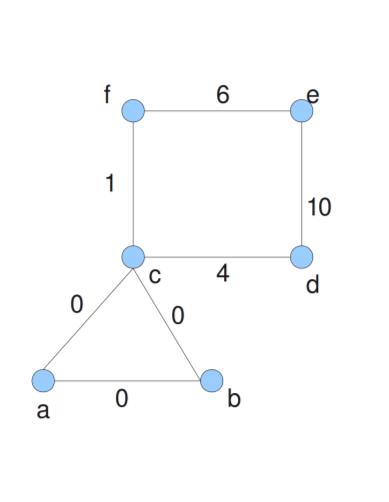
Figure 2: Gπ after iteration 1.
Figure 3: Gπ after iteration 2. Shrinking.
Figure 4: Gπ after iteration 3. Edge tight.
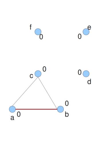
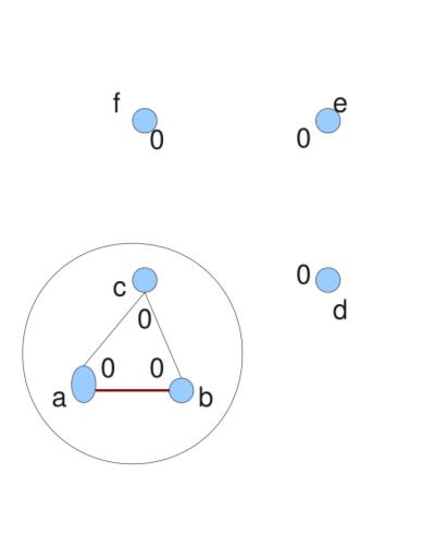
Figure 5: Gπ after iteration 4. Augment.
Figure 6: Gπ after iteration 5. Edge tight.
Figure 7: Gπ after iteration 6. Deshrink.
Figure 8: G after iteration 7. Edge tight. Some edges become slack and hence disappear from G .
π
π
Figure 9: Gπ after iteration 8. Augment. Maximum hence STOP.
1
.4 Proof
Lemma 3 The algorithm maintains the following invariants over the iterations
•
•
•
π is dual feasible
Ω is laminar
for each U ∈ Ω, HU has a hamiltonian cycle BU .
Proof Sketch. We need to check that each iteration maintains the given properties. So we do an
analysis of all the considered cases and see that in each case, this property is preserved.
If M is augmented then Ω and π don’t change.
If we shrink a blossom B in finding P then we add U = ∪
Sv to Ω. This preserves laminarity
u∈B
since nodes in G0 correspond to the maximal sets in Ω. Since we set π(U) = 0 no dual violation
happens. Moreover, B is an odd cycle and hence HU indeed contains a hamiltonian cycle for the
new set U added to Ω.
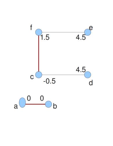
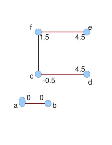
For the final case we observe that we are not adding any sets to Ω and ꢀ is chosen to ensure dual
feasiblity. Deshrinking preserves laminarity.
2
Claim 4 If M is a matching in G0 then there is a matching N in G where number of N−exposed
π
nodes is same as M−exposed nodes.
Proof: We can recursively expand the nodes in G0 and extend M using the fact that HU has a
Hamiltonian cycle for each U ∈ Ω.
2
Corollary 5 If M is a perfect matching in G0 then it can be extended to perfect matching N in
G .
π
Claim 6 If the algorithm terminates with a perfect matching then it is an optimal matching.
Proof: Let π be the feasible dual solution at the end of the algorithm. If M is a perfect matching
in G then, {x(e) = 1 if e ∈ M and x(e) = 0 otherwise}, is a feasible primal solution and x and π
π
satisfy complementary slackness conditions thus implying that both the solutions are optimal. 2
The above claims show that if the algorithm terminates then it outputs an optimum solution.
Now we establish that the algorithm indeed terminates.
Lemma 7 (Main Lemma) The algorithm terminates in O(|V |2) iterations.
Each iteration can be implemented in O(m) time with minimal data structures, Thus we have
the following theorem due to Edmonds.
Theorem 8 (Edmonds) There is a an O(n2m) time algorithm for the min cost perfect matching
problem.
As a corollary we also obtain
Corollary 9 The polytope Q(G) described by the inequalities below:
x(δ(v)) = 1 ∀v ∈ V
x(δ(U)) ≥ 1 ∀U ⊂ V, |U| ≥ 3, |U|odd
(2)
x(e) ≥ 0 ∀e ∈ E
is the convex hull of the perfect matchings in G.
Proof: The algorithm shows that for any given weights w : E → R+, the linear program min{w·x |
x ∈ Q(G)} has an integral optimum solution whenever Q(G) = ∅. Since w ≥ 0 can be assumed
w.l.o.g. so Q(G) is an integral polyhedron.
2
Now we finish the proof of the key lemma on termination. First we observe the following.
Proposition 10 In any iteration, the number of M−exposed nodes in G0 does not increase which
implies that the induced matching in G cannot decrease in size.
Proof: It is easy to see that steps (1) - (4) of the algorithm don’t increase the number of M−exposed
nodes in G0. The only non-trivial case is step (5) in which the dual value is changed. Now in this
step, recall the Edmonds Gallai decomposition and notice that A(G0) is matched only to D(G0).
The dual update in this step leaves any edge uv between D(G0) and A(G0) tight and so all the
M−edges remain tight in this step.
2
Claim 11 (Main claim) If a set U is added to Ω in some iteration (“shrinking”) then it is re-
moved from Ω (“deshrinking”) only after the matching size has increased.
Proof: When U is added to Ω, it corresponds to the blossom of an M−flower where M is the
current matching in G0. Let v be the node in G0 corresponding to U after it is shrunk. If X is the
set of M−exposed nodes then there is an X − v, M−alternating, even length path. If there is no
matching augmentation then v continues to have an X − v, M−alternating, even length path or v
is swallowed by a larger set U0 that is shrunk. In the former case, v cannot be in A(G0) and hence
cannot be “deshrunk”. In the latter case, U0 is not deshrunk before a matching augmentation and
hence U, which is inside U0, cannot be deshrunk before a matching augmentation.
2
Claim 12 Suppose iteration i has a matching augmentation and iteration j > i is the next matching
augmentation. Then between i and j, there are at most |V | shrinkings and at most |V | deshrinkings.
Proof: Let Ω be the laminar family of shrunk sets at the end of iteration i. By the previous claim,
before iteration i, we can only deshrink sets in Ω. Hence # of deshrinkings is ≤ |Ω| − |V | since we
cannot deshrink singletons. Thus the number of deshrinkings is ≤ |V |.
Similarly number of of shrinkings is at most |Ω0|−|V | where Ω0 is the laminar family just before
iteration j. Again this gives an upper bound of |V |.
2
Now lets have a look at what else can happen in an iteration other than augmentation, shrinking,
and deshrinking. In step (5), an edge uv ∈ E\E can become tight and join E . One of the
π
π
following two cases must happen since dual values are increased for nodes in D(G0), decreased for
nodes in A(G0), and unchanged for C(G0):
1
2
. u, v ∈ D(G0).
. u ∈ D(G0), v ∈ C(G0).
The following two claims take care of these cases.
Claim 13 If edge uv becomes tight in an iteration and u, v ∈ D(G0) then the next iteration is either
a shrinking iteration or an augmentation iteration.
Proof: Let X be the set of M−exposed nodes in G0. If u, v ∈ D(G0) then G0 +uv creates an X −X
M−alternating walk of odd length because D(G
0
) consists of all the vertices reachable by a walk
of even length from X. This implies that in the next iteration we have a non-empty walk leading
to an augmentation or shrinking.
2
Claim 14 If u ∈ D(G0) and v ∈ C(G0) then in G00 = G0 + uv, v is reachable from X by an
M−alternating path.
Now we can prove the key lemma. We have a total of |V | augmentation iterations. Between
2
consecutive augmentation iterations, there are at most 2|V | shrinking and deshrinking iterations.
Each other iteration is an edge becoming tight. Case 1 iterations can be charged to shrinking
iterations. Total number of case 2 iterations is at most |V | since each such iteration increases by 1,
the number of nodes reachable from X with an M−alternating path. No other iteration decreases
the number of nodes reachable before a matching augmentation. Thus the number of iterations
between augmentation is O(|V |). Hence total number of iterations is O(|V |2).

CS 598CSC: Combinatorial Optimization
Instructor: Chandra Chekuri
Lecture date: February 25, 2010
Scribe: Bill Kinnersley
1
Total Dual Integrality
Recall that if A is TUM and b, c are integral vectors, then max{cx : Ax ≤ b} and min{yb : y ≥
0
, yA = c} are attained by integral vectors x and y whenever the optima exist and are finite. This
gives rise to a variety of min-max results, for example we derived K¨onig’s theorem on bipartite
graphs. There are many examples where we have integral polyhedra defined by a system Ax ≤ b
but A is not TUM; the polyhedron is integral only for some specific b. We may still ask for the
following. Given any c, consider the maximization problem max{cx : Ax ≤ b}; is it the case that
the dual minimization problem min{yb : y ≥ 0, yA = c} has an integral optimal solution (whenever
a finite optimum exists)?
This motivates the following definition:
Definition 1 A rational system of inequalities Ax ≤ b is totally dual integral (TDI) if, for all
integral c, min{yb : y ≥ 0, yA = c} is attained by an integral vector y∗ whenever the optimum exists
and is finite.
Remark 2 If A is TUM, Ax ≤ b is TDI for all b.
This definition was introduced by Edmonds and Giles[2] to set up the following theorem:
Theorem 3 If Ax ≤ b is TDI and b is integral, then {x : Ax ≤ b} is an integral polyhedron.
This is useful because Ax ≤ b may be TDI even if A is not TUM; in other words, this is a
weaker sufficient condition for integrality of {x : Ax ≤ b} and moreover guarantees that the dual is
integral whenever the primal objective vector is integral.
Proof Sketch. Let P = {x : Ax ≤ b}. Recall that we had previously shown that the following are
equivalent:
(i) P is integral.
(ii) Every face of P contains an integer vector.
(iii) Every minimal face of P contains an integer vector.
(iv) max{cx : x ∈ P} is achieved by an integral vector whenever the optimum is finite.
Edmonds and Giles proved two more equivalent conditions:
(v) Every rational supporting hyperplane of P contains an integer vector.
(vi) If c is integral, then max{cx : x ∈ P} is an integer whenever the optimum exists and is finite.

Condition (vi) implies the theorem as follows. If Ax ≤ b is TDI and b is integral, max{cx : x ∈ P}
is an integer for all integral c whenever it is finite; this is because the dual optimum is achieved by
an integral vector y∗ (TDI property) and the objective function by∗ is integral because b is integral.
This implies that P is integral.
2
There’s an important subtlety to the definition of total dual integrality: being TDI is a property
of a system of inequalities, not a property of the corresponding polyhedron.
(1, 2)
(1, 2)
y
y
(1, 1)
(1, 1)
(2, 1)
(2, 1)
(2, 2)
(2, 2)
x
x
x ≥ 0, y ≥ 0
x + 2y ≤ 6
x ≥ 0, y ≥ 0
x + 2y ≤ 6
2x + y ≤ 6
x + y ≤ 4
2
x + y ≤ 6
x ≤ 3, y ≤ 3
We will illustrate this with an example from [3]. Consider the system Ax ≤ b drawn above on
the left. If we take the cost vector c to be (1, 1), then the primal has an optimum at (2, 2) with
value 4. The tight constraints at this vertex have normal vectors (2, 1) and (1, 2) (these are rows of
A). Therefore, in order for the dual yA = c to have an integer solution, we must be able to express
(1, 1) as an integer combination of (2, 1) and (1, 2). Since this is impossible, Ax ≤ b is not TDI.
However, suppose we add more constraints to obtain the system A0x ≤ b0 drawn above on the
right. Note that this system corresponds to the same polyhedron as Ax ≤ b. However, now we have
an additional normal vector at (2, 2) – namely, (1, 1). Thus (1, 1) is now an integer combination of
the normal vectors at (2, 2). The system A0x ≤ b0 is in fact TDI, even though it corresponds to the
same polytope as the (non-TDI) system Ax ≤ b.
The example demonstrates a necessary for a system to be TDI. We explain this in the general
context. Consider the problem max{cx : Ax ≤ b} with c integral, and assume it has a finite
optimum β. Then it is achieved by some vector x∗ in the face F defined by the intersection of
{
x : Ax ≤ b} with the hyperplane cx = β. For simplicity assume that the face F is an extreme
point/vertex of the polyhedron and let A0x∗ = b0 be the set of all inequalities in Ax ≤ b that are
tight at x∗. The dual is min{yb : y ≥ 0, yA = c}. By LP duality theory, any dual optimum solution
y corresponds to c being expressed a non-negative combination of the row vectors of A0
, in other
words c is in the cone of the row vectors of A0. If Ax ≤ b is TDI then we ask for an integral dual
optimum solution; this requires that there is an integer solution to yA0 = c, y ≥ 0. This motivates
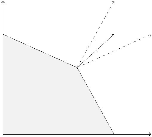
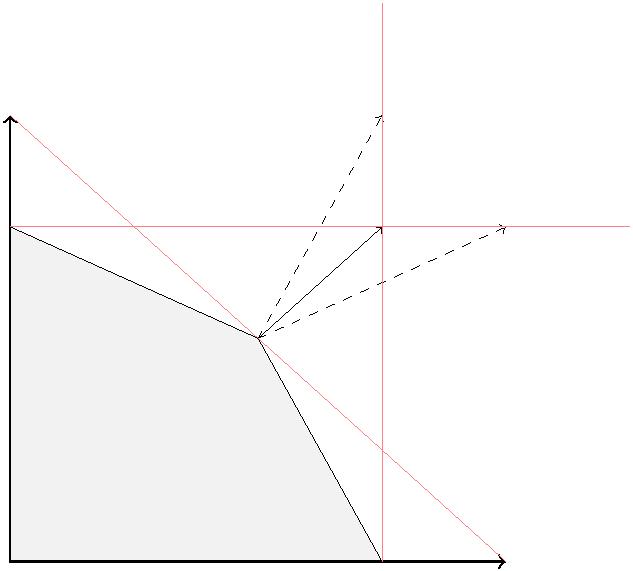
the following definition.
Definition 4 A set {a , . . . , a } of vectors in Rn is a Hilbert basis if every integral vector x ∈
1
k
P
Cone({a , . . . , a }) can be written as x =
k
i=1
µ a , µ ≥ 0, µ ∈ Z (that is, x is a non-negative
1
k
i
i
i
i
integer combination of a , . . . , a ). If the a are themselves integral, we call {a , . . . , a } an integral
1
k
i
1
k
Hilbert basis.
The following theorem is not difficult to prove with the background that we have developed.
Theorem 5 The rational system Ax ≤ b is TDI if and only if the following property is true for
each face F of P; let A0x = b0 be the set of all inequalities in Ax ≤ b that are tight/active at F,
then the rows vectors of A0 form a Hilbert basis.
Corollary 6 If the system Ax ≤ b, αx ≤ β is TDI then Ax ≤ b, αx = β is also TDI.
The example above raises the question of whether one can take any rational system Ax ≤ b
and make it TDI by adding sufficiently many redundant inequalities. Indeed that is possible, and
is based on the following theorem.
Theorem 7 Every rational polyhedral cone has a finite integral Hilbert basis.
Theorem 8 (Giles-Pulleyblank) Any rational polyhedron P has a representation Ax ≤ b such
that
(i) P = {x : Ax ≤ b},
(ii) A is integral, and
(iii) Ax ≤ b is TDI.
Moreover, b is integral if and only if P is integral.
2
The Cunningham-Marsh Theorem
Suppose we have a graph G = (V, E). Let Podd(V ) denote the family of all odd subsets of V with
size at least 3. Recall that in our study of matchings, we have examined three different systems of
inequalities.
x(δ(v)) = 1
x(δ(U)) ≥ 1
x ≥ 0
∀v ∈ V
P1 :
P2 :
P3 :
U ∈ Podd(V )
x(δ(v)) ≤ 1
∀v ∈ V
ꢀ
ꢁ
ꢁ
x(E[U]) ≤
1
2
|U|
|U|
U ∈ P
V
( )
odd
x ≥ 0
x(δ(v)) = 1
∀v ∈ V
U ∈ P
ꢀ
x(E[U]) ≤
1
2
V
( )
odd
x ≥ 0

Here P determines the matching polytope for G, while P and P determine the perfect match-
2
1
3
ing polytope.
It is not hard to see that P is not TDI. Consider K with w(e) = 1 for every edge e. In this
1
4
case, the unique optimal dual solution is y = 1 for each vertex v.
v
2
On the other hand, P and P are TDI; this was proven by Cunningham and Marsh[1]. Consider
2
3
the primal maximization and dual minimzation problems for P2 below:
ꢂ
ꢃ
X
X
1
2
maximize wx subject to
x(δ(v)) ≤ 1
minimize
yv +
z ·
|U| subject to
U
∀v ∈ V
v∈V
U∈P (V )
odd
X
ꢀ
ꢁ
x(E[U]) ≤
1
2
|U| ∀U ∈ Podd
V
( )
y + y +
zU ≥ w(ab) ∀ab ∈ E
a
b
U∈P (V )
x ≥ 0
odd
a,b∈U
y ≥ 0, z ≥ 0
By integrality of the matching polytope, the maximum value of the primal is the maximum
weight of a matching under w; by duality, this equals the minimum value of the dual. The
Cunningham-Marsh Theorem tells us that this minimum value is achieved by integral dual vectors
y∗, z∗ with the additional condition that the sets
:
∗
0 form a laminar family.
{U z > }
U
Theorem 9 (Cunningham-Marsh) The system P is TDI (as is P ). More precisely, for every
2
3
integral w, there exist integral vectors y and z that are dual feasible such that {U : z > 0} is
U
laminar and
ꢂ
ꢃ
X
X
1
2
yv +
z ·
|U| = ν(w)
U
v∈V
U∈P (V )
odd
where ν(w) is the maximum weight of a matching under w.
Exercise 10 Show that the Tutte-Berge Formula can be derived from the Cunningham-Marsh The-
orem.
Cunningham and Marsh originally proved this theorem algorithmically, but we present a differ-
ent proof from [4]; the proof relies on the fact that P2 is the matching polytope. A different proof
is given in [4] that does not assume this and in fact derives that P2 is the matching polytope as a
consequence.
Proof: We will use induction on |E| + w(E) (which is legal because w is integral). Note that if
w(e) ≤ 0 for some edge e, we may discard it; hence we may assume that w(e) ≥ 1 for all e ∈ E.
Case I: Some vertex v belongs to every maximum-weight matching under w.
Define w0 : E → Z+ by
0
( ) = ( )
w e
1
if
if
( )
e ∈ δ v
( )
w e −
e ∈ δ v
0
w e
w e
( ) = ( )
Now induct on w0. Let y0, z0 be an integral optimal dual solution with respect to w0 such that {U :
0
0 is laminar; the value of this solution is ( 0). Because appears in every maximum-weight
z > }
ν w
v
U
matching under w, ν(w0) ≤ ν(w)−1; by definition of w0, ν(w0) ≥ ν(w)−1. Thus ν(w0) = ν(w)−1.


Let y∗ agree with y0 everywhere except v, and let y∗ = y0 + 1. Let z∗ = z0. Now y∗, z∗ is a dual
v
v
feasible solution with respect to w, the solution is optimal since it has weight ν(w0) + 1 = ν(w),
and {U : z∗ > 0} is laminar since z∗ = z0.
U
Case II: No vertex belongs to every maximum-weight matching under w.
Let y, z be a fractional optimal dual solution. Observe that y = 0, since yv > 0 for some vertex
v, together with complementary slackness, would imply that every optimal primal solution covers
v, i.e. v belongs to every maximum-weight matching under w. Among all optimal dual solutions
P
ꢀ
ꢁ
y, z (with y = 0) choose the one that maximizes
zU
1
2
|U|
2. To complete the proof,
U∈P (V )
odd
we just need to show that z is integral and {U : z > 0} is laminar.
U
Suppose {U : z > 0} is not laminar; choose W, X ∈ P (V ) with z > 0, zX > 0, and
U
odd
W
W ∩X = ∅. We claim that |W ∩ X| is odd. Choose v ∈ W ∩X, and let M be a maxmimum-weight
ꢀ
ꢁ
matching under w that misses v. Since z > 0, by complementary slackness, M contains 1 |W|
W
2
edges inside W; thus v is the only vertex in W missed by M. Similarly, v is the only vertex in X
missed by M. Thus M covers W ∩X −{v} using only edges inside W ∩X −{v}, so |W ∩ X − {v}|
is even, and so |W ∩ X| is odd. Let ꢀ be the smaller of z and z ; form a new dual solution by
W
X
decreasing zW and z by ꢀ and increasing z
and z
by ꢀ (this is an uncrossing step).
X
W∩X
W∪X
We claim that this change maintains dual feasibility and optimality. Clearly z and zX are
still nonnegative. If an edge e is contained in W and X, then the sum in e’s dual constraint loses
W
2
ꢀ from zW and zX, but gains 2ꢀ from z
and z
, and hence still holds. Likewise, if e is
W∩X
W∪X
contained in W but not X (or vice-versa), the sum loses ꢀ from z but gains ꢀ from z
these changes maintained dual feasibility and did not change the value of the solution, so we still
. Thus
W
W∪X
P
ꢀ
ꢁ
2
have an optimal solution. However, we have increased
verify this), which contradicts the choice of z. Thus {U : z > 0} is laminar.
odd
zU 1 |U| (the reader should
U∈P (V )
2
odd
U
Suppose instead that z is not integral. Choose a maximal U ∈ P (V ) such that z is not an
U
integer. Let U , . . . , U be maximal odd sets contained in U such that each z > 0. (Note that
1
k
U
i
we may have k = 0.) By laminarity, U , . . . , U are disjoint. Let α = z − bz c. Form a new dual
1
k
U
U
solution by decreasing z by α and increasing each z by α.
U
U
i
We claim that the resulting solution is dual feasible. Clearly we still have z ≥ 0, and no
U
other dual variable was decreased. Thus we need only consider the edge constraints; moreover, the
only constraints affected are those corresponding to edges contained within U. Let e be an edge
contained in U. If e is contained in some Ui, then the sum in e’s constraint loses α from zU but
gains α from z , so the sum does not change. On the other hand, suppose e is not contained in
U
i
any U . By maximality of U and the U , U is the only set in P containing e. Thus before we
i
i
odd
changed zU we had z ≥ w(e); because w(e) is integral, we must still have z ≥ w(e). Hence our
U
U
new solution is dual feasible.
ꢀ
ꢁ
P
ꢀ
ꢁ
Since the Ui are disjoint, contained in U, and odd sets, 1 |U| >
k
i=1
1 |U | . Thus our new
i
2
2
solution has a smaller dual value than the old solution, which contradicts the optimality of z. It
follows that z was integral, which completes the proof.
To show that the system P is TDI, we use Corollary 6 and the fact that system P is TDI. 2
3
2
References
[
1] W. H. Cunningham and A. B. Marsh, III. A primal algorithm for optimal matching. Mathe-
matical Programming Study 8 (1978), 50–72.


[
2] J. Edmonds and R. Giles. Total dual integrality of linear inequality systems. Progress in
combinatorial optimization (Waterloo, Ont., 1982), 117–129, Academic Press, Toronto, ON,
1
984.
[
[
3] Lecture notes from Michael Goemans’s class on Combinatorial Optimization.
http://math.mit.edu/ goemans/18438/lec6.pdf. 2009.
4] A. Schrijver. Theory of Linear and Integer Programming. Wiley, 1998.
CS 598CSC: Combinatorial Optimization
Instructor: Chandra Chekuri
Lecture date: 02 March, 2010
Scribe: Ben Raichel
1
T-joins and Applications
This material is based on [1] (Chapter 5), and also [2] (Chapter 29).
Edmonds was motivated to study T-joins by the Chinese postman problem which is the follow-
ing.
Problem 1 Let G = (V, E) be an undirected graph and c : E → R be non-negative edge weights
on the edges. A Chinese postman tour is a walk that starts at some arbitrary vertex and returns to
it after traversing each edge of E. Note that an edge may be traversed more than once. The goal is
to find a postman tour of minimum total edge cost.
+
Proposition 1 If G is Eulerian then the optimal postman tour is an Eulerian tour of G and has
cost equal to c(e).
P
e∈E
Thus the interesting case is when G is not Eulerian. Let T ⊆ V be the nodes with odd degree
in G.
Fact 1 |T| is even.
Consider a postman tour and say it visits an edge x(e) times, where x(e) ≥ 1 is an integer.
Then, it is easy to see that the multigraph induced by placing x(e) copies of e is in fact Eulerian.
Conversely if x(e) ≥ 1 and x(e) ∈ Z such that the graph is Eulerian, then it induces a postman
+
P
tour of cost
c(e)x(e).
e∈E
We observe that if x(e) > 2 then reducing x(e) by 2 maintains feasibility. Thus x(e) ∈ {1, 2}
0
for each e in any minimal solution. If we consider the graph induced by x(e) = x(e)−1 we see that
each node in T has odd degree and every other node has even degree. This motivates the definition
of T-joins.
Definition 2 Given a graph, G = (V, E), and a set, T ⊆ V , a T-join is a subset J ⊆ E such that
in the graph (V, J), T is the set of nodes with odd degree.
Proposition 3 There is a T-join in G iff |K ∩ T| is even for each connected component K of G.
In particular, if G is connected then there exists a T-join iff |T| is even.
Proof: Necessity is clear. For sufficiency, assume G is connected, otherwise we can work with each
connected component separately. Let T = {v , v , . . . , v }. Let P be an arbitrary path joining v
1
and v . Then the union of the paths P , P , . . . , P induces a multigraph in which the nodes in T
2
2k
i
i
i+k
1
2
k
are the only ones with odd degree. Let x(e) be the number of copies of e in the above union. Then
x0(e) = x(e) mod 2, is the desired T-join. (Note that the pairing of the vertices was arbitrary and
hence any pairing would work.)
2
1
Proposition 4 J is a T-join iff J is the union of edge disjoint cycles and |T| paths connecting
2
disjoint pairs of nodes in T.
Proof: This is left as an exercise.
2


1
.1 Algorithm for Min-cost T-joins
Given G = (V, E), c : E → R and T ⊆ V , where |T| even, we want to find the min-cost T-join. If
all edge costs are non-negative then one can easily reduce the problem to a matching problem as
follows. Assume without loss of generality that G is connected.
1
. For each pair u, v ∈ T let w(uv) be the shortest path distance between u and v in G, with
edge length given by c. Let P be the shortest path between u and v.
uv
2
3
4
. Let H be the complete graph on T with edge weights w(uv).
. Compute a minimum weight perfect matching M in H.
. Let J = {e | e occurs in an odd number of paths Puv, uv ∈ M}. Output J.
Theorem 5 There is a strongly polynomial time algorithm to compute a min-cost T-join in a
graph, G = (V, E) with c ≥ 0.
Proof Sketch. To see the correctness of this algorithm first note that it creates a T-join since it
1
will return a collection of |T| disjoint paths, which by Proposition 4 is a T-join (Note the fourth
2
step in the algorithm is required to handle zero cost edges, and is not necessary if c > 0). It can
be seen that this T-join is of min-cost since the matching is of min-cost (and since, ignoring zero
cost edges, the matching returned must correspond to disjoint paths in G).
2
The interesting thing is that min-cost T-joins can be computed even when edge lengths can be
negative. This has several non-trivial applications. We reduce the general case to the non-negative
cost case by making the following observations.
Fact 2 If A,B are two subsets of U then |A∆B| is even iff |A| and |B| have the same parity, where
we define X∆Y as the symmetric difference of X and Y .
0
Proposition 6 Let J be a T-join and J be a T -join then J∆J is a (T∆T )-join.
0
0
0
0
Proof: Verify using the above fact that each v ∈ T∆T has odd degree and every other node has
0
even degree in J∆J .
2
0
0
0
0
Corollary 7 If J is a T -join and J∆J is a (T∆T )-join then J is a T-join.
0
Proof: Note that (T∆T )∆T = T and similarly (J∆J )∆J = J. Hence the corollary is implied
by application of the above proposition.
0
0
0
2
Given G = (V, E) with c : E → R, let N = {e ∈ E | c(e) < 0}. Let T be the set of nodes with
0
0
00
0
odd degree in G[N]. Clearly N is a T -join by definition. Let J be a (T∆T )-join in G with the
costs on edges in N negated (i.e. c(e) = |c(e)|, ∀e ∈ E).
0
0
0
Claim 8 J = J ∆N is a T-join, where N = {e ∈ E | c(e) < 0}, T = {v ∈ G[N] | δG[N](v) is odd},
0
and J is a (T∆T )-join.
0
0
0
Proof: By the above corollary, since J is a (T∆T )-join and N is a T -join, J ∆N is a (T∆T )∆T =
0
0
0
00
0
0
T-join.
2

P
0
0
|c(x)| and J, J00, and N are as defined
Claim 9 c(J) = |c|(J ) + c(N), where |c|(X) =
x∈X
above.
Proof:
0
0
00
00
c(J) = c(J ∆N) = c(J \ N) + c(N \ J )
0
0
00
00
00
=
c(J \ N) − c(J ∩ N) + c(J ∩ N) + c(N \ J )
0
0
00
00
=
c(J \ N) + |c|(J ∩ N) + c(N) = |c|(J ) + c(N).
2
0
0
00
0
Corollary 10 J = J ∆N is a min cost T-join in G iff J is a min cost (T∆T )-join in G with
edge costs |c|, where N = {e ∈ E | c(e) < 0}, T = {v ∈ G[N] | δG[N](v) is odd}, and J00 is a
0
0
(T∆T )-join.
Proof Sketch. By using the last claim, necessity is clear since c(N) is a constant and hence when
0
0
c(J) is minimized so is |c|(J ). To use the same argument for sufficiency, one must argue that for
0
0
0
00
any T-join, J, we have that J = J ∆N for some (T∆T )-join, J .
2
The above corollary gives a natural algorithm to solve the general case by first reducing it
to the non-negative case. In the algorithm below, let c : E → R, |c| : E → R such that
+
|
c|(e) = |c(e)|, G be the graph with the weight function |c|, N = {e ∈ E | c(e) < 0}, and
c|
|
0
T = {v ∈ G[N] | δ
(v) is odd}.
G[N]
0
00
1
. Compute a (T∆T )-join , J , on G using the algorithm above for c ≥ 0
c|
|
0
0
. Output J = J ∆N.
2
Theorem 11 There is a strongly polynomial time algorithm for computing a min-cost T-join in a
graph, even with negative costs on the edges.
0
Proof: We know the above algorithm outputs a T-join by Claim 8. Since J was computed on
G , which has non-negative edge weights, by the proof of Theorem 5, J is a min-cost T-join.
0
0
0
|
c|
Hence by Corollary 10 J is a min-cost T-join.
2
1
.2 Applications
1
.2.1 Chinese Postman
We saw earlier that a min-cost postman tour in G is the union of E and a T-join where T is the
set of odd degree nodes in G. Hence we can compute a min-cost postman tour.
1
.2.2 Shortest Paths and Negative lengths
In directed graphs the well known Bellman-Ford and Floyd-Warshall algorithms can be used to
check whether a given directed graph, D = (V, A), has negative length cycles or not in O(mn) and
O(n3) time respectively. Moreover, if there is no negative length cycle then the shortest s-t path
can be found in the same time. However, one cannot use directed graph algorithms for undirected
graphs when there are negative lengths, since bi-directing an undirected edge creates a negative
length cycle. However, we can use T-join techniques.
Proposition 12 An undirected graph, G = (V, E), with c : E → R has a negative length cycle iff
an ∅-join has negative cost.
-
5
-10
s
t
2
1
1
Figure 1: An example of a graph with a negative cost ∅-join
Proposition 13 If G has no negative length cycle then the min-cost {s, t}-join gives an s-t shortest
path.
Remark 14 It is important to first check for negative length cycles before finding an {s, t}-join.
Theorem 15 There is a strongly polynomial time algorithm that given an undirected graph, G(V, E),
with c : E → R, either outputs a negative length cycle or an s-t shortest path.
Proof Sketch. We first compute a min-cost ∅-join. By Proposition 12 we know that if this ∅-join
has negative cost then we can produce a negative length cycle. Otherwise, we know there is no
negative length cycle and hence by Proposition 13 we can compute a min-cost {s, t}-join in order
to find an s-t shortest path. (In each case the T-join can be computed using the algorithm from
the previous section.)
2
1
.2.3 Max-cut in planar graphs
Since one can compute min-cost T-joins with negative costs, one can compute max-cost T-joins as
well. The max-cut problem is the following.
Problem 2 Given an undirected graph with non-negative edge weights, find a partition of V into
(S, S \ V ) so as to maximize w(δ(S)).
Max-cut is NP-hard in general graphs, but Hadlock showed how T-joins can be used to solve it
in polynomial time for planar graphs. A basic fact is that in planar graphs, cuts in G correspond
to collections of edge disjoint cycles in the dual graph G∗. Thus to find a max-cut in G we compute
∗
∗
a max ∅-join in G where the weight of an edge in G is the same as its corresponding edge in the
primal.

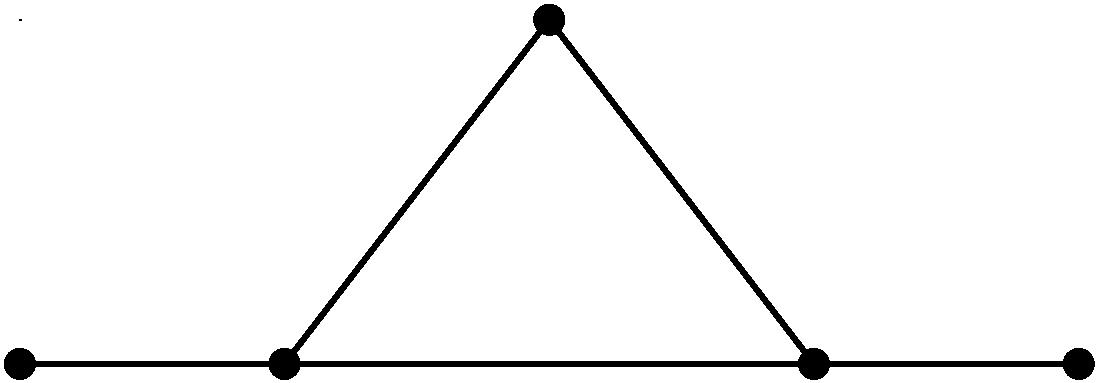
G
G*
Figure 2: A planar graph, G, in black, and its dual, G∗, in dashed red.
1
.2.4 Polyhedral aspects
The following set of inequalities can be shown to determine the characteristic vectors of the set of
T-joins in a graph G.
0
≤ x(e) ≤ 1
x(δ(U) \ F) − x(F) ≥ 1 − |F|
U ⊆ V, F ⊆ δ(U), |U ∩ T| + |F| is odd
References
[
1] W.J. Cook, W.H. Cunningham, W.R. Pulleyblank, and A. Schrijver. Combinatorial Optimiza-
tion. Wiley, 1998.
[
2] A. Schrijver. Theory of Linear and Integer Programming (Paperback). Wiley, 1998.
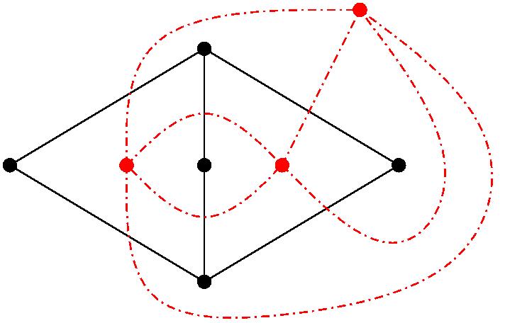
CS 598CSC: Combinatorial Optimization
Instructor: Chandra Chekuri
Lecture date: March 4, 2010
Scribe: Vineet Abhishek
The presentation here is based on [1] and [2].
1
Introduction to Matroids
Matroids (formally introduced by Whitney in 1935) are combinatorial structures that capture the
abstract properties of linear independence defined for vector spaces.
Definition 1 A matroid M is a tuple (S, I), where S is a finite ground set and I ⊆ 2S (the power
set of S) is a collection of independent sets, such that:
1
2
3
. I is nonempty, in particular, ∅ ∈ I,
. I is downward closed; i.e., if X ∈ I and Y ⊆ X, then Y ∈ I,
. If X, Y ∈ I, and |X| < |Y |, then ∃y ∈ Y \X such that X + y ∈ I.
Exercise 2 Show that the third property in Definition 1 can be replaced by the following: if X, Y ∈
I, |Y | = |X| + 1, then ∃y ∈ Y \X such that X + y ∈ I.
Example 3 (Vector Matroid) Let M be a m × n matrix with entries in some field F and vi
be the ith column of M, viewed as a vector in the vector space Fm. Let S = {1, 2, . . . , n} and
I = {I : I ⊆ S, {v }
are linearly independent} (under the usual definition of linear independence
i
i∈I
in linear algebra). Then M = (S, I) is a matroid. To see this, notice that properties 1 and 2 of
Definition 1 are trivially satisfied. To show property 3, suppose X, Y ∈ I and |X| < |Y |. If there
is no y ∈ Y \X such that X + y ∈ I, then Y is in the span of {v }
. Hence, |Y | ≤ |X| which is
x∈X
x
a contradiction.
Example 4 (Graphic Matroid) Let G = (V, E) be an undirected multi-graph (loops allowed).
Let I = {I : I ⊆ E, I induces a forest in G}. Then M = (E, I) is a matroid. Again, the first
two properties of Definition 1 are easy to verify. To show property 3, suppose X, Y ∈ I such that
|
X| < |Y |. Both X and Y induce forests in G. Let V , V , . . . , V
be the vertex sets of the
k(X)
1
2
connected components in G[X] (G restricted to the edge set X). Here, k(X) denotes the number
of connected components in G[X]. Each connected component is a tree. Hence, if there is an
edge y ∈ Y that connects two different components of G[X] then G[X + y] is again a forest and
we are done. If not, then every edge y ∈ Y have its both ends in the same component of G[X].
Thus, the number of connected components in G[Y ], denoted by k(Y ), is at least k(X). Thus,
|
X| = |V | − k(X) ≥ |V | − k(Y ) = |Y |, which is a contradiction.
Example 5 (Uniform Matroid) Let M = (S, I), where S is any finite nonempty set, and I =
{
I : I ⊆ S, |I| ≤ k} for some positive integer k. Then M is a matroid.
Example 6 (Partition Matroid) Let S , S , . . . , S be a partition of S and k , k , . . . , k be pos-
1
2
n
1
2
n
itive integers. Let I = {I : I ⊆ S, |I ∩ S | ≤ k for all 1 ≤ i ≤ n}. Then M = (S, I) is a
i
i
matroid.

Example 7 (Laminar Matroid) Let F be a laminar family on S (i.e., if X, Y ∈ F then X, Y ⊆
S; and either X ∩ Y = ∅, or X ⊆ Y , or Y ⊆ X) such that each x ∈ S is in some set X ∈ F.
For each X ∈ F, let k(X) be a positive integer associated with it. Let I = {I : I ⊆ S, |I ∩ X| ≤
k(X) ∀X ∈ F}. Then M = (S, I) is a matroid. Notice that laminar matroids generalize partition
matroids, which in turn generalize uniform matroids.
Exercise 8 Verify Example 7.
Example 9 (Transversal Matroid) Let G = (V, E) be a bipartite graph with bipartition V and
1
V . let I = {I : I ⊆ V , ∃ a matching M in G that covers I}. Then M = (V , I) is a matroid.
2
1
1
Example 10 (Matching Matroid) Let G = (V, E) be an undirected graph. Let I = {I : I ⊆
V, ∃ a matching M in G that covers I}. Then M = (V, I) is a matroid.
Exercise 11 Verify Examples 9 and 10.
1
.1 Base, Circuit, Rank, Span and Flat
Let M = (S, I) be a matroid.
Definition 12 A set X ⊆ S such that X ∈/ I is called a dependent set of M.
Definition 13 A loop is an element x ∈ S such that {x} is dependent.
Notice that a loop cannot appear in any sets in I and can be effectively removed from S.
Definition 14 A base is an inclusion wise maximal set in I.
Proposition 15 If B and Bb are bases of M then |B| = |Bb|.
Proof: If |B| < |Bb| then from Definition 1, ∃x ∈ Bb\B such that B + x ∈ I, contradicting the
maximality of B.
2
Notice that the notion of base here is similar to that of a basis in linear algebra.
Lemma 16 Let B and Bb be bases of M and x ∈ Bb\B. Then ∃y ∈ B\Bb such that Bb − x + y is a
base of M.
Proof: Since Bb−x ∈ I and |Bb−x| < |B|, ∃y ∈ B\Bb such that Bb−x+y ∈ I. Then |Bb−x+y| = |B|,
implying that Bb − x + y is a base of M.
2
Definition 17 Let M = (S, I) be a matroid. Given Sb ⊆ S, let Ib = {I : I ⊆ Sb, I ∈ I}. Then
c = (b b) is also a matroid and is referred to as the restriction of
to b.
M
S, I
M
S
Definition 18 Given M = (S, I) and Sb ⊆ S, Bb is a base for Sb if Bb is a base of Mc, where Mc is
a restriction of M to Sb.
Proposition 19 Given M = (S, I), let B ⊆ X be a base for X. Then for any Y ⊇ X, there exist
a base Bb for Y that contains B.
Proof: Notice that B is independent in the restriction of M to Y (henceforth independent in Y ).
Let Bb be the maximal independent set in Y that contains B. Since all maximal independent sets
have same size, Bb is a base of Y .
2
Definition 20 Given M = (S, I), a circuit is a minimal dependent set (i.e., an inclusion wise
minimal set in 2S\I). Thus, if C is a circuit then ∀x ∈ C, C − x ∈ I.
The definition of a circuit is related to graph theory in the following sense: if M is the graphic
matroid of a graph G, then the circuits of M are the cycles of G. Single element circuits of a
matroid are loops; if M is a graphic matroid of a graph G, then the set of loops of M is precisely
the set of loops of G.
Lemma 21 Let C and C be two circuits such that C = C and x ∈ C ∩ C . Then for every
1
2
1
2
1
2
x ∈ C \C there is a circuit C such that x ∈ C and C ⊆ C ∪ C − x. In particular, C ∪ C − x
1
1
2
1
1
2
1
2
contains a circuit.
Proof: Notice that C \C is nonempty (and so is C \C ), otherwise, C ⊆ C . Since C = C , C
1
2
2
1
1
2
1
2
1
is a strict subset of C , contradicting the minimality of C .
2
2
Let C ∪ C − x contain no circuits. Then B = C ∪ C − x is independent, and hence, a base
1
2
1
2
for C ∪C (since it is maximal). Also, |B| = |C ∪C |−1. Since C ∩C is an independent set, we
1
2
1
2
1
2
can find a base Bb for C ∪ C that contains C ∩ C . Then |Bb| = |B| = |C ∪ C | − 1. Since C \ C
1
2
1
2
1
2
1
2
and C \ C are both non-empty, this is possible only if either C ⊆ Bb or C ⊆ Bb, contradicting
2
1
1
2
that Bb is a base. Hence, C ∪ C − x must contain a circuit.
1
2
Now let x ∈ C \C . Let B be a base for C ∪ C that contains C − x , and B be a base
1
1
2
1
1
2
1
1
2
for C ∪ C that contains C − x. Clearly, x ∈/ B and x ∈/ B . If x ∈/ B then B + x must
1
2
2
1
1
2
1
2
2
1
have a circuit and we are done. If x ∈ B , then from Lemma 16, there exists xb ∈ B \B such that
1
2
1
2
b =
+
is a base for
. Notice that = , otherwise
b. Thus,
b and
B
B − x
xb
C ∪ C
xb
x
C ⊆ B
x ∈/ B
2
1
1
2
2
1
b +
contains the circuit satisfying the condition of Lemma 21.
B
x
2
1
Corollary 22 Let M = (S, I) be a matroid. If X ∈ I and y ∈/ X then either X + y ∈ I or there
is a unique circuit C in X + y. Moreover, for each yb ∈ C, X + y − yb ∈ I.
Proof: If X +y ∈/ I, then it must contain a circuit C . Assume there is another circuit C ⊆ X +y,
1
2
and C = C . Since X ∈ I, both C and C must contain y. From Lemma 21, C ∪C −y contains
1
2
1
2
1
2
a circuit. But this is a contradiction since C ∪C −y ⊆ X. Hence, X +y contains a unique circuit,
1
2
call it C. Now, if for some yb ∈ C, X +y −yb ∈/ I, then X +y −yb is dependent and contains a circuit
b. However, b = since
b, contradicting that is unique.
C
C
C
yb ∈/ C
C
2
Corollary 23 If B and Bb are bases. Let xb ∈ Bb\B, then ∃x ∈ B\Bb such that B + xb − x is a base.
Proof Sketch. Follows from Corollary 22.
2
Definition 24 Let M = (S, I) be a matroid. The rank function, denoted by r , of M is r
:
M
M
2
S → Z , where for X ⊆ S, r (X) is the size of a maximum independent set contained in X.
+
M
Note that the above definition assigns a unique number to each set X since all maximal inde-
pendent sets contained in X have the same cardinality.
Proposition 25 Given a matroid M = (S, I), the rank function rM has the following properties:
1
. 0 ≤ rM(X) ≤ |X| for all X ⊆ S.
2
. rM is submodular; i.e., for any X, Y ⊆ S, r (X ∪ Y ) + r (X ∩ Y ) ≤ r (X) + r (Y ).
M
M
M
M
Proof: Property 1 is by the definition of r . To show the second property, we use the equivalent
M
definition of submodularity; i.e., we show that if X ⊆ Y and z ∈ S, then r (X + z) − r (X) ≥
M
M
r (Y + z) − r (Y ). First notice that for any X ⊆ S and z ∈ S, r (X + z) ≤ r (X) + 1. Thus,
M
M
M
M
we only need to show that if r (Y +z)−r (Y ) = 1 then r (X +z)−r (X) = 1 for any X ⊆ Y .
M
M
M
M
If r (Y +z) −r (Y ) = 1, then every base B of Y +z contains z. Let Bb be a base of X. Since
M
M
¯
¯
b
b
X ⊆ Y + z, from Proposition 19, there exists a base B of Y + z such that B ⊇ B. Then B + z is
independent, implying r (X + z) − r (X) = 1 as Bb + z is a base in X + z.
2
M
M
Definition 26 Let M = (S, I) be a matroid. For any X ⊆ S, the span of X, denoted by
span (X), is defined as span (X) = {y : y ∈ S, r (X + y) = r (X)}. A set X ⊆ S is
M
spanning if span (X) = S.
M
M
M
M
Exercise 27 Prove the following properties about the span function spanM : 2S → 2S.
•
•
If T, U ⊆ S and U ⊆ span (T) then span (U) ⊆ span (T).
M
M
M
If T ⊆ S, t ∈ S \ T and s ∈ span (T + t) \ span (T) then t ∈ span (T + s).
M
M
M
Definition 28 Let M = (S, I) be a matroid. A subset X ⊆ S is a flat of M iff spanM (X) = X.
Exercise 29 Prove the following properties about flats.
•
•
If F and F are flats then F ∩ F is a flat.
1
2
1
2
If F is a flat and t ∈ S \ F and F
0
is a smallest flat containing + then there is no flat 00
F
t
F
with F ⊂ F00 ⊂ F0.
Remark 30 We showed basic properties of bases, circuits, rank, span and flats of a matroid. One
can show that a matroid can alternatively be specified by defining its bases or circuits or rank or
span or flats that satisfy these properties. We refer the reader to [2].
References
[
1] J. Lee. “Matroids and the greedy algorithm”. In A First Course in Combinatorial Optimiza-
tion, Ch. 1, 49–74, Cambridge University Press, 2004.
[
2] A. Schrijver. Combinatorial optimization: polyhedra and efficiency, Chapter 39 (Vol B),
Springer, 2003.
C S 598C SC :C om binatorial O p tim izatio n
In stru ctor: C handra C hekuri
L ectu re d ate: M arch 9, 2009
S crib e: S reeram K annan
1
Maximum Weight Independent Set in a Matroid, Greedy Algo-
rithm, Independence and Base Polytopes
1
.1 More on Matroids
W e saw the definition of base,circuit,ran k,sp an and flat ofm a troidsla stlectu re.W e begin this
lectu re by studying som e m ore basic p rop erties ofa m a troid.
E xercise 1 Show that a setI ⊆ S is independent in a m a tro id M iff ∀y ∈ I, there e x ists a flatF
su ch thatI− y ⊆ F and y ∈ F .
D efi n ition 2 A m a tro id M = (S,I) is defi n ed as con n ected ifr (U )+ r (S\U ) > r (S) for
M
M
M
each U ⊆ S,U = ∅. E quivalently, for each s,t∈ S,s= t, there is a circuit containing bo th s,t.
1
.2 Operations on a Matroid
1
.2 .1 D ual
Given a m a troid M = (S,I)its dualm a troid M∗ = (S,I∗)is defined as follow s:
is spanningini.e.,
I∗ {I ∈ S | S\I
=
M,
r
(
S\I
)=
r
( )
S }.
M
M
E xercise 3 V erify that(S,I∗)is in deed a m atroid.
The following facts are easy to p rove:
1
. M∗∗ = M.
2
. Bisa b ase ofM∗iff S\Bisa b ase ofM.
3
. r (U )= |U | + r (S\U )− r (S)
M∗
M
M
R em ark 4 H aving an in depen den ce or rank oracle fo r M im plie s one has it for M∗ too .
E xercise 5 P rove thatM is con n ected if and only ifM∗ is .
Hint:Use th e third p rop erty fro m ab ove.
1 .2 .2 D eletio n
D efi n ition 6 G iven a m a tro id M = (S,I)and e∈ S,deletin g e fro m M generates a n ew m a tro id
M0
=
= (
S − e,I0),
(1)
M\e
w here I0 = {I − e|I ∈ I}. For Z ⊆ S, the m a tro id M\Z is obtain ed s im ilarly by restrictin g the
m a tro id M to S\Z.

1 .2 .3 C on traction
D efi n ition 7 G iven a m a tro id M = (S,I)and e∈ S, the con traction of the m a tro id w ith respect
to e is defined asM/e= (M∗\e)∗, i.e., it is obtained by deletin g e in th e dualand takin g its dual.
S im ilarly for a setZ ⊆ S,we can s im ilarly define M/Z = (M∗\Z)∗
Itisin stru ctive to view th e con traction op eration fro m a grap h th eoretic p ersp ective.Ifeisa
loop,M/e= M\e,else M/e= (S − e,I0) w here
I0 {I ∈ S − e|I e∈ I}.
=
+
For the case of contracting a subsetZ,we can take a b ase X ⊆ Z and M /Z = (S\Z,I0),w here
I0 {I ∈ S\Z|I∪ Z ∈ I}.
=
Also
r
(X )= r (X ∪ Z)− r (Z)
M/Z
M
M
E xercise 8 Show that
M/{e,e } = (M/e )/e = (M/e )/e .
(2)
1
2
1
2
2
1
1 .2 .4 M inor
Simila r to grap h min ors,m a troid min ors can be defined,and th ey play anim p ortant rolein
ch aracterizing th e type ofm a troids.
D efi n ition 9 A m a tro id M0 is a m inor ofa m a tro id M ifM0 is obtain ed fro m M by a sequ en ce
of contractions and deletion s.
1
.3 Maximum Weight Independent Set in a Matroid
M a troids have som eim p ortant algorith mic p rop erties,th e sim plest one being th at th e p roblem
of determining th e m axim um weightindep endent setin a m a troid can be solved using a greed y
algorithm.The m axim um weightindependent set problemis stated as follow s:Given M = (S,I)
and w:S → R,output
arg m axw(I).
(3)
I∈I
1
.3 .1 G reed y A lgorith m
The greed y algorithm can be stated as follow s:
. Discard alle∈ S w here w(e)≤ 0 oreisaloop.
. LetS = {e,...,e } su ch thatw(e )≥ w(e )...≥ w(e ).
1
2
1
n
1
2
n
3
. X ← ∅.
4.Fori = 1 to n,do
if(X + e ∈ I) then X ← X + e .
i
i
5.O utputX .
T he above algorith m had to sp ecifi cally take care ofloops and edges with non-negativeweigh ts.
An equivalent algorith m without this hassleis:
1
. LetS = {e,...,e } su ch thatw(e )≥ w(e )...≥ w(e ).
1
n
1
2
n
2
. X ← ∅.
3.Fori = 1 to n,do
if(X + e ∈ I) and w(X + e )≥ w(X ),th en X ← X + e .
i
i
i
4.O utputX .
T h eorem 10 The greed y algo rith m outputs an optim um solu tion to th e m axim um w eight indepen-
dent set problem .
P ro of: Withoutloss of generality,assu m e w(e)> 0,∀e∈ S and that there a re noloop s.
C la im 11 T here e x ists an optim um solu tion that contains e1.
A ssuming this claimis tru e,we can u seinduction to sh ow th at greed y algorith m has to yield an
optim um solution.Thisis because the greedy algorith mis recursively finding an optim um solution
in the m a troid M0 = (S − e,I0) w here I0 = {I− e |I ∈ I0}.
1
To prove the claim,letI∗ be an optim um solution.Ife ∈ I∗,we are done,else,we can see that
1
I∗
∃
+
is notindep endent,oth erwise ( ∗ +
)
( ∗).T hus ∗ + con tainsa circuit,and hence
w I e > w I
e
1
I
e
1
1
e ∈ I∗
su ch th at
I − e e ∈ I
∗
+
w I − e
(S ee C orolla ry 22in th ela stlectu re).( ∗
+
e
)
1
≥ w I
( ∗)
1
sin ce w(e ) has th ela rg est weight am ong all the elem en tsin th e set.T hus th ereis an optim um
1
solution I∗ − e+ e that containse .
2
1
1
R em ark 12 Ifallw eights are n on -n egative th en it is easy to see that the greed y algo rith m outputs
a ba se ofM. W e can adapt th e greed y algo rith m to solve th e m axim um w eight ba se problem by
m akin g allw eights non-negative by adding ala rge constant to each of the weights. T hus m ax-w eight
ba se problem , and equ ivalen tly m in -cost base problem ca n be solved (by takin g th e w eights to be the
n egative of the co sts).
R em ark 13 K ru skal’s algo rith m for finding th e m axim um w eight spanning tree ca n be in terp reted
as a specialca se of the greed y algo rith m fo r m atroids w hen applied to th e graphic m a tro id co rre-
spon din g to th e graph.
1 .3 .2 O racles for a M atro id
Sin ce the set ofallindep endence sets could be exp onentialin |S|,itisin feasible to use this rep -
resen ta tion.In stead we resort to one of the two oraclesin ord er to effi ciently solve optimization
p roblem s:
•
•
Anindep endence oracle that given A ⊆ S,returns w hetherA ∈ I or not.
A ran k oracle that given A ⊆ S,returnsrM(A).
T hese tw o oracles a re equivalentin th e sen se th at one can be recovered fro m th e oth erin
polynomialtim e.
1
.4 Matroid Polytopes
Edm onds utilized th e G reed y algorithmin p roving th e following th eorem :
T h eorem 14 The follow ing polytope is th e con vex hullof the ch a ra cteristic vecto rs of the in de-
pendent sets ofa m a tro id M = (S,I)w ith ran k fu n ction rM:2S → Z+,
x(A)≤ r (A) ∀A ⊆ S,
M
x(A)≥ 0.
Also, the sy stem of inequalitie s d escribed above is TDI.
P ro of: W e willsh ow that the above sy stem ofinequalitiesis TD I (Totally D ualIn teg ral),which
willin tu rnim ply that the polytop eisin tegralsin ce r (.)isinteger valued.
M
Let us consider the prim aland duallinear program s for som ein tegralweight vectorw:S → Z.
W e willsh ow th at th e solution picked by G reed y algorith mis th e optim alsolution for prim alby
producing a dualsolution th at a ttains th e sam e value.Altern ately we could sh ow th at th e dual
solution and the prim alsolution picked by G reed y satisfy com plem en tary slack n ess.
X
Prim al: m ax
w(e)x(e)
e∈S
x(A)≤ r(A),∀ A ⊆ S
x ≥ 0
X
D ual: min
r(A)y(A)
A ∈S
X
y(A)≥ w(e),∀e∈ S
A :e∈A
y ≥ 0
LetS = {e,...,e } su ch thatw(e )≥ w(e )...≥ w(e )≥ 0,sin ce setting w(e )= 0 w henever
1
n
1
2
n
i
w(e )< 0 does not alter the solution of the prim alor dual. D efine A = {e,...,e } with A = ∅.
i
j
1
j
0
Itis easy to see thatr(A )= r(A
)+ 1iff eis picked by G reed y.C onsid er th e following dual
j
j−1
j
solution
y(Aj) = w(e )− w(ej+1),j< n
j
=
w(e ),j= n
n
y(A) = 0,ifA = Aj for som e j
C la im 15 y is dualfea sible.
Clearly,y ≥ 0.Sin ce w(e )≥ w(e )∀j,for any e ,
j
j−1
i
X
X
y(A) =
y(Ai)
A :e ∈A
j≥i
nX−1
i
=
=
{w(ej)− w(ej+1)} + w(en)
j=i
w(e )
i
D efine I = {i|eispicked by G reed y}.Aswe n oted earlier,i∈ I ⇐⇒ r(A )= r(Ai−1)+ 1.
i
i
C la im 16
X
X
w(ei)=
r(A)y(A)
i∈I
A ⊆S
X
X
w(ei) =
w(e )(r(A )− r(Ai−1))
i
i
i∈I
i∈I
Xn
=
w(e )(r(A )− r(Aj−1))
j
j
j=1
nX−1
=
w(e )y(A )+
(w(ej)− w(ej+1))r(Aj)
n
n
j=1
Xn
=
=
y(A )r(A )
j
j
j=1
X
r(A)y(A)
A ⊆S
T husy has to be dualoptim al,and the solution produced by G reed y has to be prim aloptim al.
This m eans th at th e dualoptim alsolutionisin tegralw henever wisin tegral, and th erefo re the
sy stemisTD I.
2
C o ro llary 17 The ba se polytope ofM = (S,I), i.e., the con vex hullof the bases ofM is d eter-
m in ed by
x(A) ≤ r(A),∀A ⊆ S,
x(S) = r(S)
x ≥ 0
1 .4 .1 Spanning Set P olytope
A nother polytop e asso ciated with a m a troidis the spanning set polytop e,whichis the convex hull
of theincid en ce vectors of all spanning sets.
T h eorem 18 The spanning set polytope ofa m a tro id M = (S,I)w ith ran k fu n ction r is d eter-
M
m in ed by
0
≤ x(e)≤ 1,∀e∈ S
x(U )≥ r (S)− r (S\U ),∀U ⊆ S.
M
M
P roof:A given setA ⊆ Sis spanningin Miff S\Aisindep endentin M∗.T husx ∈ Pspanning(M)
independence
iff 1− x ∈ P (M∗).Now,by th e relation betw een th e ranks ofdualm a troids,
r
(U )= |U | + r (S\U )− r (S).
M∗
M
M
Thus1− x ∈ Pindependence(M∗)iff
1
− x ≥ 0,
|
U | − x(U ) ≤ r (U )= |U | + r (S\U )− r (S),
M∗
M
M
which m atches the statem ent ofthe th eorem .
2
1 .4 .2 S ep aration O ra cle
W e have now d etermin ed th at th eindep endence polytop e of a m a troidis given by th elin ear
conditionsx ≥ 0 and x(U )≤ r (U ),U ⊆ S.The greed y algorith m allows us to optimize over the
M
polytop e and by th e equivalen ce betw een optimization and sep aration,th ereisa polynomialtim e
sep aration oracle for the polytop e.Itisin stru ctive to considerit explicitly.
For the sep aration p roblem,given a test vector w:S → R,we n eed to find outif w ∈
independence
P
(M).W e can easily test for non-negativity.To test the second condition,itis suffi cient
to ch eck that min
(r (A)− w(A))≥ 0.In fact any violatedinequalityin th elinear system can
A ⊆S
M
be found by con stru cting th e set
U = arg min (r (A)− w(A)).
M
A ⊆S
D efinef:2S → R,w heref(A)= r (A)−w(A).fisa subm odular set function sincer(.)is the
M
subm odular rank function and −w(.)ism odular.T husifw e can minimize an a rbitra ry subm odular
function sp ecifi ed by a value oracle,we can use th e sam e for separating over a m a troid polytop e.
H ow ever,th ereisa m o re effi cient algorith m for separating over theindep endence polytopes given
by C unningham.S ee[1]for details .
References
[1]Lex Schrijv er,“C om bin atorialO ptimization:Polyhedra and Effi cien cy,Vol. B,” Sprin ger-
Verlag 2003.
Massachusetts Institute of Technology
8.433: Combinatorial Optimization
Michel X. Goemans
Handout 9
March 20th, 2009
1
4
. Lecture notes on matroid optimization
4
.1 Definition of a Matroid
Matroids are combinatorial structures that generalize the notion of linear independence in
matrices. There are many equivalent definitions of matroids, we will use one that focus on
its independent sets. A matroid M is defined on a finite ground set E (or E(M) if we want
to emphasize the matroid M) and a collection of subsets of E are said to be independent.
The family of independent sets is denoted by I or I(M), and we typically refer to a matroid
M by listing its ground set and its family of independent sets: M = (E, I). For M to be a
matroid, I must satisfy two main axioms:
(I1) if X ⊆ Y and Y ∈ I then X ∈ I,
(I2) if X ∈ I and Y ∈ I and |Y | > |X| then ∃e ∈ Y \ X : X ∪ {e} ∈ I.
In words, the second axiom says that if X is independent and there exists a larger independent
set Y then X can be extended to a larger independent by adding an element of Y \X. Axiom
(I ) implies that every maximal (inclusion-wise) independent set is maximum; in other words,
2
all maximal independent sets have the same cardinality. A maximal independent set is called
a base of the matroid.
Examples.
•
•
One trivial example of a matroid M = (E, I) is a uniform matroid in which
I = {X ⊆ E : |X| ≤ k},
for a given k. It is usually denoted as Uk,n where |E| = n. A base is any set of
cardinality k (unless k > |E| in which case the only base is |E|).
A free matroid is one in which all sets are independent; it is Un,n.
Another is a partition matroid in which E is partitioned into (disjoint) sets E , E , · · · , E
1
2
l
and
I = {X ⊆ E : |X ∩ E | ≤ k for all i = 1, · · · , l},
i
i
for some given parameters k , · · · , k . As an exercise, let us check that (I ) is satisfied.
1
l
2
If X, Y ∈ I and |Y | > |X|, there must exist i such that |Y ∩ E | > |X ∩ E | and this
i
i
means that adding any element e in E ∩ (Y \ X) to X will maintain independence.
Observe that M would not be a matroid if the sets E were not disjoint. For example,
i
i
if E = {1, 2} and E = {2, 3} with k = 1 and k = 1 then both Y = {1, 3} and
1
2
1
2
X = {2} have at most one element of each E , but one can’t find an element of Y to
i
add to X.

4
. Lecture notes on matroid optimization
March 20th, 2009
2
•
Linear matroids (or representable matroids) are defined from a matrix A, and this is
where the term matroid comes from. Let E denote the index set of the columns of
A. For a subset X of E, let AX denote the submatrix of A consisting only of those
columns indexed by X. Now, define
I = {X ⊆ E : rank(AX) = |X|},
i.e. a set X is independent if the corresponding columns are linearly independent. A
base B corresponds to a linearly independent set of columns of cardinality rank(A).
Observe that (I1) is trivially satisfied, as if columns are linearly independent, so is a
subset of them. (I2) is less trivial, but corresponds to a fundamental linear algebra
property. If A has full column rank, its columns span a space of dimension |X|, and
X
similarly for Y , and therefore if |Y | > |X|, there must exist a column of A that is not
Y
in the span of the columns of A ; adding this column to A increases the rank by 1.
X
X
A linear matroid can be defined over any field F (not just the reals); we say that the
matroid is representable over F. If the field is F2 (field of 2 elements with operations
(mod 2)) then the matroid is said to be binary. If the field is F3 then the matroid is
said to be ternary.
For example, the binary matroid corresponding to the matrix
1
1 0
A = 1 0 1
0
1 1
corresponds to U2,3 since the sum of the 3 columns is the 0 vector when taking com-
ponents modulo 2. If A is viewed over the reals or over F3 then the matroid is the free
matroid on 3 elements.
Not every matroid is linear. Among those that are linear, some can be represented
over some fields F but not all. For example, there are binary matroids which are not
ternary and vice versa (for example, U2,4 is ternary but not binary). Matroids which
can be represented over any field are called regular.
•
•
Here is an example of something that is not a matroid. Take a graph G = (V, E), and
let I = {F ⊆ E : F is a matching}. This is not a matroid since (I ) is not necessarily
2
satisfied ((I ) is satisfied1, however). Consider, for example, a graph on 4 vertices and
1
let X = {(2, 3)} and Y = {(1, 2), (3, 4)}. Both X and Y are matchings, but one cannot
add an edge of Y to X and still have a matching.
There is, however, another matroid associated with matchings in a (general, not nec-
essarily bipartite) graph G = (V, E), but this time the ground set of M corresponds to
V . In the matching matroid, I = {S ⊆ V : S is covered by some matching M}. In
this definition, the matching does not need to cover precisely S; other vertices can be
covered as well.
1
When (I1) alone is satisfied, (E, I) is called an independence system.

4
. Lecture notes on matroid optimization
March 20th, 2009
3
•
A very important class of matroids in combinatorial optimization is the class of graphic
matroids (also called cycle matroids). Given a graph G = (V, E), we define independent
sets to be those subsets of edges which are forests, i.e. do not contain any cycles. This
is called the graphic matroid M = (E, I), or M(G).
(I ) is clearly satisfied. To check (I ), first notice that if F is a forest then the number of
1
2
connected components of the graph (V, F) is given by K(V, F) = |V | − |F|. Therefore,
if X and Y are 2 forests and |Y | > |X| then K(V, Y ) < K(V, X) and therefore there
must exist an edge of Y \ X which connects two different connected components of X;
adding this edge to X results in a larger forest. This shows (I ).
2
If the graph G is connected, any base will correspond to a spanning tree T of the graph.
If the original graph is disconnected then a base corresponds to taking a spanning tree
in each connected component of G.
A graphic matroid is a linear matroid. We first show that the field F can be chosen to
be the reals. Consider the matrix A with a row for each vertex i ∈ V and a column for
each edge e = (i, j) ∈ E. In the column corresponding to (i, j), all entries are 0, except
for a 1 in i or j (arbitrarily) and a −1 in the other. To show equivalence between the
0
original matroid M and this newly constructed linear matroid M , we need to show
that any independent set for M is independent in M0 and vice versa. This is left as an
exercise.
In fact, a graphic matroid is regular; it can be represented over any field F. To obtain
a representation for a field F, one simply needs to take the representation given above
for R and simply view/replace all −1 by the additive inverse of 1 (i.e. by p − 1 for
F ).
p
4
.1.1 Circuits
A minimal (inclusionwise) dependent set in a matroid is called a circuit. In a graphic matroid
M(G), a circuit will be the usual notion of a cycle in the graph G; to be dependent in the
graphic matroid, one needs to contain a cycle and the minimal sets of edges containing a
cycle are the cycles themselves. In a partition matroid, a circuit will be a set C ⊆ E with
i
|
C ∩ E | = k + 1.
i
i
By definition of a circuit C, we have that if we remove any element of a circuit then we
get an independent set. A crucial property of circuit is given by the following property,
Theorem 4.1 (Unique Circuit Property) Let M = (E, I) be a matroid. Let S ∈ I and
e such that2 S + e ∈/ I. Then there exists a unique circuit C ⊆ S + e.
The unicity is very important. Indeed, if we consider any f ∈ C where C is this unique
circuit then we have that C +e−f ∈ I. Indeed, if C +e−f was dependent, it would contain
0
a circuit C which is distinct from C since f / C , a contradiction.
∈
0
2
For a set S and an element e, we often write S + e for S ∪ {e} and S − e for S \ {e}.

4
. Lecture notes on matroid optimization
March 20th, 2009
4
As a special case of the theorem, consider a graphic matroid. If we add an edge to a
forest and the resulting graph has a cycle then it has a unique cycle.
Proof:
Suppose S+e contains more than one circuit, say C and C with C = C . By minimality
1
2
1
2
of C and C , we have that there exists f ∈ C \ C and g ∈ C \ C . Since C − f ∈ I (by
1
2
1
2
2
1
1
minimality of the circuit C ), we can extend it to a maximal independent set X of S + e.
1
Since S is also independent, we must have that |X| = |S| and since e ∈ C −f, we must have
1
that X = S + e − f ∈ I. But this means that C ⊆ S + e − f = X which is a contradiction
2
since C is dependent.
4
2
Exercise 4-1. Show that any partition matroid is also a linear matroid over F = R. (No
need to give a precise matrix A representing it; just argue its existence.)
Exercise 4-2. Prove that a matching matroid is indeed a matroid.
Exercise 4-3. Show that U2,4 is representable over F3.
Exercise 4-4. Consider the linear matroid (over the reals) defined by the 3 × 5 matrix:
1
2 1 0
1
A = 1 2 0 1 −1 .
1
2 0 1 −1
The ground set E = {1, 2, 3, 4, 5} has cardinality 5, corresponds to the columns of A, and
the independent sets are the set of columns which are linearly independent (over the reals).
1
2
3
.Give all bases of this matroid.
.Give all circuits of this matroid.
.Choose a base B and an element e not in B, and verify the unique circuit property for
B + e.
Exercise 4-5. Given a family A , A , · · · , A of sets (they are not necessarily disjoint), a
1
2
n
transversal is a set T such that T = {a , a , · · · , a }, the a ’s are distinct, and a ∈ A for all
1
2
n
i
i
i
i. A partial transversal is a transversal for A , A , · · · , A for some subfamily of the A ’s.
i
i
i
k
i
1
2
Show that the family of all partial transversals forms a matroid (on the ground set E = ∪A ).
i
(Hint: Think of bipartite matchings.)
Exercise 4-6. Let M = (E, I) be a matroid. Let k ∈ N and define
Ik = {X ∈ I : |I| ≤ k}.
Show that M = (E, I ) is also a matroid. This is known as a truncated matroid.
k
k
4
. Lecture notes on matroid optimization
March 20th, 2009
5
Exercise 4-7. A family F of sets is said to be laminar if, for any two sets A, B ∈ F, we
have that either (i) A ⊆ B, or (ii) B ⊆ A or (iii) A∩B = ∅. Suppose that we have a laminar
family F of subsets of E and an integer k(A) for every set A ∈ F. Show that (E, I) defines
a matroid (a laminar matroid) where:
I = {X ⊆ E : |X ∩ A| ≤ k(A) for all A ∈ F}.
4
.2 Matroid Optimization
Given a matroid M = (E, I) and a cost function c : E → R, we are interested in finding
P
an independent set S of M of maximum total cost c(S) =
problem.
c(e). This is a fundamental
e∈S
If all c(e) ≥ 0, the problem is equivalent to finding a maximum cost base in the matroid.
If c(e) < 0 for some element e then, because of (I ), e will not be contained in any optimum
1
solution, and thus we could eliminate such an element from the ground set. In the special case
of a graphic matroid M(G) defined on a connected graph G, the problem is thus equivalent
to the maximum spanning tree problem which can be solved by a simple greedy algorithm.
This is actually the case for any matroid and this is the topic of this section.
The greedy algorithm we describe actually returns, for every k, a set Sk which maximizes
c(S) over all independent sets of size k. The overall optimum can thus simply be obtained
by outputting the best of these. The greedy algorithm is the following:
.
.
.
Sort the elements (and renumber them) such that c(e ) ≥ c(e ) ≥ · · · ≥ c(e|M|)
1
2
S = ∅, k=0
0
For j = 1 to |E|
.
if S + e ∈ I then
k
.
j
k ← k + 1
.
.
S ← S
+ ej
k
k−1
s ← e
k
j
.
Output S , S , · · · , S
1
2
k
Theorem 4.2 For any matroid M = (E, I), the greedy algorithm above finds, for every k,
an independent set S of maximum cost among all independent sets of size k.
k
Proof:
Suppose not. Let S = {s , s , · · · , s } with c(s ) ≥ c(s ) ≥ · · · ≥ c(s ), and
k
1
2
k
1
2
k
suppose T has greater cost (c(T ) > c(S )) where T = {t , t , · · · , t } with c(t ) ≥ c(t ) ≥
k
k
k
k
1
2
k
1
2
·
· · ≥ c(t ). Let p be the first index such that c(t ) > c(s ). Let A = {t , t , · · · , t } and
k
p
p
1
2
p
B = {s , s , · · · , s }. Since |A| > |B|, there exists t ∈/ B such that B + t ∈ I. Since
1
2
p−1
i
i
c(t ) ≥ c(t ) > c(s ), t should have been selected when it was considered. To be more
i
p
p
i
precise and detailed, when t was considered, the greedy algorithm checked whether t could
i
i
be added to the current set at the time, say S. But since S ⊆ B, adding t to S should have
i
resulted in an independent set (by (I )) since its addition to B results in an independent set.
1
This gives the contradiction and completes the proof.
4
4
. Lecture notes on matroid optimization
March 20th, 2009
6
Observe that, as long as c(s ) ≥ 0, we have that c(S ) ≥ c(Sk−1). Therefore, to find a
k
maximum cost set over all independent sets, we can simply replace the loop
k
.
For j = 1 to |E|
by
.
For j = 1 to q
where q is such that c(e ) ≥ 0 > c(eq+1), and output the last Sk.
q
For the maximum cost spanning tree problem, the greedy algorithm reduces to Kruskal’s
algorithm which considers the edges in non-increasing cost and add an edge to the previously
selected edges if it does not form a cycle.
One can show that the greedy algorithm actually characterizes matroids. If M is an
independence system, i.e. it satisfies (I1), then M is a matroid if and only if the greedy
algorithm finds a maximum cost set of size k for every k and every cost function.
Exercise 4-8. We are given n jobs that each take one unit of processing time. All jobs
are available at time 0, and job j has a profit of c and a deadline d . The profit for job
j
j
j will only be earned if the job completes by time dj. The problem is to find an ordering
of the jobs that maximizes the total profit. First, prove that if a subset of the jobs can be
completed on time, then they can also be completed on time if they are scheduled in the
order of their deadlines. Now, let E(M) = {1, 2, · · · , n} and let I(M) = {J ⊆ E(M) : J
can be completed on time }. Prove that M is a matroid and describe how to find an optimal
ordering for the jobs.
4
.3 Rank Function of a Matroid
Similarly to the notion of rank for matrices, one can define a rank function for any matroid.
The rank function of M, denoted by either r(·) or rM (·), is defined by:
rM : 2E → : rM (X) = max{|Y | : Y ⊆ X, Y ∈ I}.
N
Here are a few specific rank functions:
•
•
For a linear matroid, the rank of X is precisely the rank in the linear algebra sense of
the matrix AX corresponding to the columns of A in X.
For a partition matroid M = (E, I) where
I = {X ⊆ E : |X ∩ E | ≤ k for i = 1, · · · , l}
i
i
(the Ei’s forming a partition of E) its rank function is given by:
X
l
r(X) =
min(|E ∩ X|, k ).
i
i
i=1
4
. Lecture notes on matroid optimization
March 20th, 2009
7
•
For a graphic matroid M(G) defined on graph G = (V, E), the rank function is equal
to:
rM(G)(F) = n − K(V, F),
where n = |V | and K(V, F) denotes the number of connected components (including
isolated vertices) of the graph with edges F.
The rank function of any matroid M = (E, I) has the following properties:
(R1) 0 ≤ r(X) ≤ |X| and is integer valued for all X ⊆ E
(R2) X ⊆ Y ⇒ r(X) ≤ r(Y ),
(R3) r(X) + r(Y ) ≥ r(X ∩ Y ) + r(X ∪ Y ).
The last property is called submodularity and is a key concept in combinatorial optimization.
It is clear that, as defined, any rank function satisfies (R ) and (R ). Showing that the rank
1
2
function satisfies submodularity needs a proof.
Lemma 4.3 The rank function of any matroid is submodular.
Proof:
Consider any two sets X, Y ⊆. Let J be a maximal independent subset of
X ∩ Y ; thus, |J| = r(X ∩ Y ). By (I ), J can be extended to a maximal (thus maximum)
2
indenpendent subset of X, call it J . We have that J ⊆ J ⊆ X and |J | = r(X).
X
X
X
Furthermore, by maximality of J within X ∩ Y , we know
J \ Y = J \ J.
(1)
X
X
Now extend JX to a maximal independent set JXY of X ∪ Y . Thus, |JXY | = r(X ∪ Y ).
In order to be able to prove that
r(X) + r(Y ) ≥ r(X ∩ Y ) + r(X ∪ Y )
or equivalently
|
JX| + r(Y ) ≥ |J| + |JXY |,
we need to show that r(Y ) ≥ |J| + |J | − |J |. Observe that J ∩ Y is independent (by
XY
X
XY
(I )) and a subset of Y , and thus r(Y ) ≥ |J ∩ Y |. Observe now that
1
XY
JXY ∩ Y = JXY \ (JX \ Y ) = JXY \ (JX \ J),
the first equality following from the fact that JX is a maximal independent subset of X and
the second equality by (1). Therefore,
r(Y ) ≥ |JXY ∩ Y | = |JXY \ (JX \ J)| = |JXY | − |JX| + |J|,
proving the lemma.
4
4
. Lecture notes on matroid optimization
March 20th, 2009
8
4
.3.1 Span
The following definition is also motivated by the linear algebra setting.
Definition 4.1 Given a matroid M = (E, I) and given S ⊆ E, let
span(S) = {e ∈ E : r(S ∪ {e}) = r(S)}.
Observe that S ⊆ span(S). We claim that r(S) = r(span(S)); in other words, if adding
an element to S does not increase the rank, adding many such elements also does not increase
the rank. Indeed, take a maximal independent subset of S, say J. If r(span(S)) > |J| then
there exists e ∈ span(S) \J such that J +e ∈ I. Thus r(S +e) ≥ r(J +e) = |J| +1 > |J| =
r(S) contradicting the fact that e ∈ span(S).
Definition 4.2 A set S is said to be closed if S = span(S).
Exercise 4-9. Given a matroid M with rank function r and given an integer k ∈ N, what
is the rank function of the truncated matroid M (see Exercise 4-6 for a definition).
k
Exercise 4-10. What is the rank function of a laminar matroid, see exercise 4-7?
4
.4 Matroid Polytope
Let
X = {χ(S) ∈ {0, 1}|E| : S ∈ I}
denote the incidence (or characteristic) vectors of all independent sets of a matroid M =
(E, I), and let the matroid polytope be defined as conv(X). In this section, we provide
a complete characterization of conv(X) in terms of linear inequalities. In addition, we
illustrate the different techniques proposed in the polyhedral chapter for proving a complete
description of a polytope.
Theorem 4.4 Let
P = {x ∈ R|E| : x(S) r(S)
≤
∀ ⊆
S
E
xe ≥ 0
∀e ∈ E}
P
where x(S) :=
xe. Then conv(X) = P.
e∈S
It is clear that conv(X) ⊆ P since X ⊆ P. The harder part is to show that P ⊆ conv(X).
In the next three subsections, we provide three different proofs based on the three techniques
to prove complete polyhedral descriptions.
4
. Lecture notes on matroid optimization
March 20th, 2009
9
4
.4.1 Algorithmic Proof
Here we provide an algorithmic proof based on the greedy algorithm. From conv(X) ⊆ P,
we know that
max{cT x : x ∈ X} = max{cT x : x ∈ conv(X)} ≤ max{cT x : x(S) ≤ r(S) S ⊆ E
x ≥ 0
e ∈ E}.
e
Using LP duality, we get that this last expression equals:
P
P
Our goal now is, for any cost function c, to get an independent set S and a dual feasible
min{
r(S)yS :
y ≥ c(e) ∀e ∈ E
∈
S
S
S
S:e
y ≥ 0
S ⊆ E}.
S
P
solution y such that cT χ(S) =
Consider any cost function c. We know that the maximum cost independent set can be
obtained by the greedy algorithm. More precisely, it is the last set S returned by the greedy
r(S)yS which proves that conv(X) = P.
S
k
algorithm when we consider only those elements up to e where c(e ) ≥ 0 ≥ c(eq+1). We
q
need now to exhibit a dual solution of the same value as S . There are exponentially many
q
k
variables in the dual, but this is not a problem. In fact, we will set most of them to 0.
For any index j ≤ k, we have S = {s , s , · · · , s }, and we define U to be all elements in
j
1
2
j
j
our ordering up to and excluding s , i.e. U = {e , e , · · · , e } where e = s . In other
j+1
j
1
2
l
l+1
j+1
words, U is all the elements in the ordering just before s . One important property of U
j
j
j+1
is that
r(U ) = r(S ) = j.
j
j
Indeed, by independence r(S ) = |S | = j, and by (R ), r(U ) ≥ r(S ). If r(U ) > r(S ),
j
j
1
j
j
j
j
there would be an element say e ∈ U \S such that S ∪{e } ∈ I. But the greedy algorithm
p
j
j
j
p
would have selected that element (by (I )) contradicting the fact that e ∈ U \ S .
1
p
j
j
Set the non-zero entries of y in the following way. For j = 1, · · · , k, let
S
yUj = c(sj) − c(sj+1),
where it is understood that c(sk+1) = 0. By the ordering of the c(·), we have that yS ≥ 0 for
all S. In addition, for any e ∈ E, we have that
X
Xk
yS =
yUj = c(st) ≥ c(e),
S:e∈S
j=t
where t is the least index such that e ∈ U (implying that e does not come before s in the
t
ordering). This shows that y is a feasible solution to the dual. Moreover, its dual value is:
t
X
Xk
Xk
Xk
Xk
r(S)yS =
r(Uj)yUj
=
j(c(sj)−c(sj+1)) =
(j−(j−1))c(sj) =
c(s ) = c(S ).
j
k
S
j=1
j=1
j=1
j=1
This shows that the dual solution has the same value as the independent set output by the
greedy algorithm, and this is true for all cost functions. This completes the algorithmic
proof.
4
. Lecture notes on matroid optimization
March 20th, 2009
10
4
.4.2 Vertex Proof
Here we will focus on any vertex x of
P = {x ∈ R|E| : x(S) r(S)
≤
∀ ⊆
S
E
xe ≥ 0
∀e ∈ E}
and show that x is an integral vector. Since x({e}) ≤ r({e}) ≤ 1, we get that x ∈ {0, 1}
|E|
and thus it is the incidence vector of an independent set.
Given any x ∈ P, consider the tight sets S, i.e. those sets for which x(S) = r(S). The
next lemma shows that these tight sets are closed under taking intersections or unions. This
lemma is really central, and follows from submodularity.
Lemma 4.5 Let x ∈ P. Let
F = {S ⊆ E : x(S) = r(S)}.
Then
S ∈ F, T ∈ F ⇒ S ∩ T ∈ F, S ∪ T ∈ F.
Observe that the lemma applies even if S and T are disjoint. In that case, it says that ∅ ∈ F
(which is always the case as x(∅) = 0 = r(∅)) and S ∪ T ∈ F.
Proof:
The fact that S, T ∈ F means that:
r(S) + r(T) = x(S) + x(T).
(2)
P
Since x(S) =
xe, we have that
e∈S
x(S) + x(T) = x(S ∩ T) + x(S ∪ T),
(3)
i.e. that the function x(·) is modular (both x and −x are submodular). Since x ∈ P, we know
that x(S ∩ T) ≤ r(S ∩ T) (this is true even if S ∩ T = ∅) and similarly x(S ∪ T) ≤ r(S ∪ T);
this implies that
x(S ∩ T) + x(S ∪ T) ≤ r(S) + r(T).
By submodularity, we have that
r(S ∩ T) + r(S ∪ T) ≤ r(S) + r(T).
(4)
(5)
Combining (2)–(5), we get
r(S) + r(T) = x(S) + x(T) = x(S ∩ T) + x(S ∪ T) ≤ r(S ∩ T) + r(S ∪ T) ≤ r(S) + r(T),
and therefore we have equality throughout. This implies that x(S ∩ T) = r(S ∩ T) and
x(S ∪ T) = r(S ∪ T), i.e. S ∩ T and S ∪ T in F.
4
To prove that any vertex or extreme point of P is integral, we first characterize any face
of P. A chain C is a family of sets such that for all S, T ∈ C we have that either S ⊆ T or
T ⊆ S (or both if S = T).
4
. Lecture notes on matroid optimization
March 20th, 2009
11
Theorem 4.6 Consider any face F of P. Then there exists a chain C and a subset J ⊆ E
such that:
F = {x ∈ R|E| : x(S) r(S)
≤
∀ ⊆
S
E
x(C) = r(C) ∀C ∈ C
x ≥ 0
∀e ∈ E \ J
e
x = 0
∀e ∈ J.}
By Theorem 3.5 of the polyhedral notes, we know that any face is characterized
e
Proof:
by setting some of the inequalities of P by equalities. In particular, F can be expressed as
F = {x ∈ R|E| : x(S) r(S)
≤
∀ ⊆
S
E
x(C) = r(C) ∀C ∈ F
x ≥ 0
∀e ∈ E \ J
e
x = 0
∀e ∈ J.}
e
where J = {e : x = 0 for all x ∈ F} and F = {S : x(S) = r(S) for all x ∈ F}. To prove the
e
theorem, we need to argue that the system of equations:
x(C) = r(C) ∀C ∈ F
can be replaced by an equivalent (sub)system in which F is replaced by a chain C. To be
equivalent, we need that
span(F) = span(C)
where by span(L) we mean
span(L) := span{χ(C) : C ∈ L}.
Let C be a maximal subchain of F, i.e. C ⊆ F, C is a chain and for all S ∈ F \ C, there
exists C ∈ C such that S ⊆ C and C ⊆ S. We claim that span(C) = span(F).
Suppose not, i.e. H = span(F) where H := span(C). This means that there exists
S ∈ F \ C such that χ(S) ∈/ H but S cannot be added to C without destroying the chain
structure. In other words, for any such S, the set of ’chain violations’
V (S) := {C ∈ C : C ⊆ S and S ⊆ C}
is non-empty. Among all such sets S, choose one for which |V (S)| is as small as possible
(|V (S)| cannot be 0 since we are assuming that V (S) = ∅ for all possible S). Now fix some
set C ∈ V (S). By Lemma 4.5, we know that both C ∩ S ∈ F and C ∪ S ∈ F. Observe that
there is a linear dependence between χ(C), χ(S), χ(C ∪ T), χ(C ∩ T):
χ(C) + χ(S) = χ(C ∪ S) + χ(C ∩ S).
This means that, since χ(C) ∈ H and χ(S) ∈/ H, we must have that either χ(C ∪ S) ∈/ H
or χ(C ∩ S) ∈/ H (otherwise χ(S) would be in H). Say that χ(B) ∈/ H where B si either
C ∪ S or C ∩ S. This is a contradiction since |V (B)| < |V (S)|, contradicting our choice of
S. Indeed, one can see that V (B) ⊂ V (S) and C ∈ V (S) \ V (B).
4
As a corollary, we can also obtain a similar property for an extreme point, starting from
Theorem 3.6.
4
. Lecture notes on matroid optimization
March 20th, 2009
12
Corollary 4.7 Let x be any extreme point of P. Then there exists a chain C and a subset
J ⊆ E such that x is the unique solution to:
x(C) = r(C) ∀C ∈ C
x = 0
e
∀e ∈ J.
From this corollary, the integrality of every extreme point follows easily. Indeed, if the
chain given in the corollary consists of C ⊂ C ⊂ C the the system reduces to
1
2
p
x(C \ Ci−1) = r(Ci) − r(Ci−1) i = 1, · · · , p
i
x = 0
∀e ∈ J,
e
where C = ∅. For this to have a unique solution, we’d better have |C \ C \ J| ≤ 1 for all
0
i and the values for the resulting x ’s will be integral.
i
i−1
e
4
.4.3 Facet Proof
Our last proof of Theorem 4.4 focuses on the facets of conv(X).
First we need to argue that we are missing any equalities. Let’s focus on the (interesting)
case in which any singleton set is independent: {e} ∈ I for every e ∈ E. In that case
dim(conv(X)) = |E| since we can exhibit |E| + 1 affinely independent points in X: the
0
vector and all unit vectors χ({e}) for e ∈ E. Thus we do not need any equalities. See
exercise 4-11 if we are not assuming that every singleton set is independent.
Now consider any facet F of conv(X). This facet is induced by a valid inequality αT x ≤ β
P
where β = max{
α : I ∈ I}. Let
e∈I
e
X
O = {I ∈ I :
αe = β},
e∈I
i.e. O is the set of all independent sets whose incidence vectors belong to the face. We’ll
show that there exists an inequality in opur description of P which is satisfied at equality
by the incidence vectors of all sets I ∈ O.
We consider two cases. If there exists e ∈ M such that α < 0 then I ∈ O implies that
e
e ∈/ I, implying that our face F is included in the face induced by x ≥ 0 (which is in our
e
description of P).
For the other case, we assume that for all e ∈ E, we have α ≥ 0. We can further assume
e
α > 0 since otherwise F is trivial. Now, define S as
that α
:= max
max
e∈E
e
S = {e ∈ E : αe = αmax}.
Claim 4.8 For any I ∈ O, we have |I ∩ S| = r(S).
This means that the face F is contained in the face induced by the inequality x(S) ≤ r(S)
and therefore we have in our description of P one inequality inducing each facet of conv(X).
Thus we have a complete description of conv(X).
4
. Lecture notes on matroid optimization
March 20th, 2009
13
To prove the claim, suppose that |I ∩ S| < r(S). Thus I ∩ S can be extended to an
independent set X ∈ I where X ⊆ S and |X| > |I ∩ S|. Let e ∈ X \ (I ∩ S); observe
that e ∈ S by our choice of X. Since α > 0 we have that I + e ∈/ I, thus there is a
e
circuit C ⊆ I + e. By the unique circuit property (see Theorem 4.1), for any f ∈ C we have
I + e − f ∈ I. But C \ S = ∅ since (I ∩ S) + e ∈ I, and thus we can choose f ∈ C \ S. The
cost of I + e − f satisfies:
c(I + e − f) = c(I) + c(e) − c(f) > c(I),
contradicting the definition of O.
4
.5 Facets?
Now that we have a description of the matroid polytope in terms of linear inequalities, one
may wonder which of these (exponentially many) inequalities define facets of conv(X).
For simplicity, let’s assume that r({e}) = 1 for all e ∈ E (e belongs to some independent
set). Then, every nonnegativity constraint defines a facet of P = conv(X). Indeed, the 0
vector and all unit vectors except χ({e}) constitute |E| affinely independent points satisfying
x = 0. This mean that the corresponding face has dimension at least |E| − 1 and since the
e
dimension of P itself is |E|, the face is a facet.
We now consider the constraint x(S) ≤ r(S) for some set S ⊆ E. If S is not closed (see
Definition 4.2) then x(S) ≤ r(S) definitely does not define a facet of P = conv(X) since it
is implied by the constraints x(span(S)) ≤ r(S) and x ≥ 0 for e ∈ span(S) \ S.
e
Another situation in which x(S) ≤ r(S) does not define a facet is if S can be expressed
as the disjoint union of U = ∅ and S \ U = ∅ and r(U) + r(S \ U) = r(S). In this case, the
inequality for S is implied by those for U and for S \ U.
Definition 4.3 S is said to be inseparable if there is no U with ∅ = U ⊂ S such that
r(S) = r(U) + r(S \ U).
From what we have just argued, a necessary condition for x(S) ≤ r(S) to define a facet
of P = conv(X) is that S is closed and inseparable. This can be shown to be sufficient as
well, although the proof is omitted.
As an example, consider a partition matroid with M = (E, I) where
I = {X ⊆ E : |X ∩ E | ≤ k for all i = 1, · · · , l},
i
i
for disjoint E ’s. Assume that k ≥ 1 for all i. The rank function for this matroid is:
i
i
X
l
r(S) =
min(k , |S ∩ E |).
i
i
i=1
For a set S to be inseparable, there must exist (i) i ∈ {1, · · · , l with S ⊆ E , and (ii) |S ∩E |
i
i
is either ≤ 1 or > k for every i. Furthermore, for S ⊆ E to be closed, we must have that if
i
i
4
. Lecture notes on matroid optimization
March 20th, 2009
14
|
S ∩ E | > k then S ∩ E = E . Thus the only sets we need for the description of a partition
i
i
i
i
matroid polytope are (i) sets S = E for i with |E | > k and (ii) singleton sets {e} for e ∈ E.
i
The partition matroid polytope is thus given by:
i
i
P = {x ∈ R|E| : x(Ei) ki
≤
i
1,
∈ { · · · } | |
, l : E > k
i
i
0
≤ x ≤ 1 e ∈ E}.
e
As another example, take M to be the graphic matroid M(G). For a set of edges F ⊆ E
to be inseparable, we need that the subgraph (V, F) has only one non-trivial (i.e. with more
than 1 vertex) connected component; indeed, if we partition F into the edge sets F , · · · , F
P
1
c
c
i=1
of the (c non-trivial) connected components, we have that r(F) =
r(F ) and thus c
i
must be 1 for F to be inseparable. Given a set F of edges, its span (with respect to the
graphic matroid) consists of all the edges with both endpoints within the same connected
component of F; these are the edges whose addition does not increase the size of the largest
forest. Thus, for F to be inseparable and closed, we must have that there exists a vertex
set S ⊆ V such that F = E(S) (E(S) denotes all the edges with both endpoints in S)
and (S, E(S)) is connected. Thus the forest polytope (convex hull of all forests in a graph
G = (V, E)) is given by:
P = {x ∈ R|E| : x(E(S))
≤ | | −
S
1 S V :E(S) connected
⊆
0
≤ xe
e ∈ E}.
P
(As usual, x(E(S)) denotes
a very large number of inequalities.
From this, we can also easily derive the spanning tree polytope of a graph, namely the
convex hull of incidence vectors of all spanning trees in a graph. Indeed, this is a face of
the forest polytope obtained by replacing the inequality for S = V (x(E) ≤ |V | − 1) by an
equality:
xe.) Observe that this polyhedral description still has
e∈E(S)
| | −
P = {x ∈ R|E| : X(E) = V
1
x(E(S)) ≤ |S| − 1 S ⊂ V :E(S) connected
≤ xe e ∈ E}.
0
Exercise 4-11. Let M = (E, I) be a matroid and let S = {e ∈ E : {e} ∈ I}. Show that
dim(conv(X)) = |S| (where X is the set of incidence vectors of indpendent sets) and show
that the description for P has the required number of linearly independent equalities.
Exercise 4-12. Let M = (E, I) be a matroid and let P be the corresponding matroid
polytope, i.e. the convex hull of characteristic vectors of independent sets. Show that two
independent sets I and I are adjacent on P if and only if either (i) I ⊆ I and |I |+1 = |I |,
1
2
1
2
1
2
or (ii) I ⊆ I and |I | + 1 = |I |, or (iii) |I \ I | = |I \ I | = 1 and I ∪ I ∈/ I.
2
1
2
1
1
2
2
1
1
2
CS 598CSC: Combinatorial Optimization
Instructor: Chandra Chekuri
Lecture date: 03/11/2010
Scribe: Alina Ene
1
Matroid Polytope
In the previous lecture we saw that for a matroid M = (S, I) the following system of inequalities
determines the convex hull of the independent sets of M (i.e., sets in I):
x(U) ≤ r (U)
U ⊆ S
e ∈ S
M
x(e) ≥ 0
where r (·) is the rank function of M. The proof was based on a dual fitting technique via the
M
Greedy algorithm for a maximum weight independent set problem.
In this lecture, we will give a different primal proof that is built on uncrossing. This is based
on [2].
Theorem 1 Let x be an extreme point of the polytope
(
x(U) ≤ r (U)
U ⊆ S
e ∈ S
(∗)
M
x(e) ≥ 0
Then there is some e ∈ S such that x(e) ∈ {0, 1}.
The following corollary follows by induction from Theorem 1. We leave a formal proof as an
exercise.
Corollary 2 The system of inequalities (∗) determine the independent set polytope of M = (S, I).
Now we turn our attention to the proof of Theorem 1.
Proof of Theorem 1. Let x be an extreme solution for the polytope (∗). Suppose that M has
M
a loop e. Since r ({e}) = 0, it follows that x(e) = 0 and we are done. Therefore we may assume
that M does not have any loops and thus the polytope (∗) is full dimensional1. Now suppose that
x(e) ∈ (0, 1) for all elements e ∈ S. Let n denote the number of elements in S. Let
F = {U | U ⊆ S, x(U) = rM (U)}
Differently said, F is the set of all sets whose constraints are tight at x (i.e., sets whose constraints
are satisfied with equality by the solution x).
Before proceeding with the proof, we note that the submodularity for the rank function r (·)
M
implies that F has the following “uncrossing” property.
1A polytope is full dimensional if it has an interior point, i.e., a point x that does not satisfy any of the constraints
with equality. Consider x such that, for all e, x(e) = ꢀ for some 0 < ꢀ < 1/|S|. Clearly, x(e) > 0 for any e. For any
set U, we have x(U) = ꢀ|U| < 1. If M does not have any loops, r (U) ≥ 1 for all sets U. Thus M is full-dimensional
M
if there are no loops.


Lemma 3 If A, B ∈ F then A ∩ B and A ∪ B are in F.
Proof: Let A and B be two sets in F; thus x(A) = r (A) and x(B) = r (B). It follows from the
M
M
submodularity of the rank function that
x(A) + x(B) = r (A) + r (B) ≥ r (A ∩ B) + r (A ∪ B)
M
M
M
M
Additionally,
x(A) + x(B) = x(A ∩ B) + x(A ∪ B)
Therefore x(A ∩ B) + x(A ∪ B) ≥ r (A ∩ B) + r (A ∪ B). Since x(A ∩ B) ≤ r (A ∩ B) and
M
M
M
x(A ∪ B) ≤ r (A ∪ B), it follows that x(A ∩ B) = r (A ∩ B) and x(A ∪ B) = r (A ∪ B). Thus
M
A ∩ B and A ∪ B are also in F.
M
M
2
Let χ(U) denote the characteristic vector of U. Since x is a vertex solution, (∗) is full dimensional,
and x(e) = 0 for all e, there is a collection {U , U , . . . , U } of n sets such that x satisfies the
1
2
n
constraint corresponding to each U with equality (i.e., x(U ) = r (U ) for 1 ≤ i ≤ n) and the
i
i
M
i
vectors χ(U ), . . . , χ(U ) are linearly independent. Therefore the set {χ(U) | U ∈ F} has n linearly
1
n
independent vectors.
For a set A ⊆ 2S, let span(A) denote span({χ(U) | U ∈ A}), where χ(U) is the characteristic
vector of U.
Lemma 4 There exists a laminar family C ⊆ F such that span(C) = span(F). Moreover, C is a
chain, i.e., for any two sets A, B ∈ C, either A ⊆ B or B ⊆ A.
Assuming Lemma 4, we can complete the proof of Theorem 1 as follows. Let C be the chain
guaranteed by Lemma 4. Since span(C) = span(F), there exists a chain C0 ⊆ C such that |C0| = n
and x is the unique solution to the system
x(U) = rM (U)
U ∈ C0
Let C0 = {A , A , . . . , A }; wlog, A ⊂ A ⊂ · · · ⊂ A . Let A = ∅. Suppose that there exists an
1
2
n
1
2
n
0
i such that |A \ A | = 1, and let e ∈ A \ A . Now we claim that we must have x(e) ∈ {0, 1}.
i
i−1
i
i−1
To see why this is true, note that we have
x(e) = x(Ai) − x(Ai−1) = r (A ) − r (Ai−1)
M
i
M
Since r (A ) − r (A ) is an integer and rM (Ai−1) ≤ r (A ) ≤ r (A ) + 1, it follows that
M
i
M
i−1
M
i
M
i−1
r (A ) − r (A ) ∈ {0, 1}. But this contradicts the fact that x(e) ∈ (0, 1). Therefore we may
M
i
M
i−1
assume that |A \ A | ≥ 2. But then |S| ≥ 2n, which is a contradiction.
i
i−1
Finally, we turn our attention to the proof of Lemma 4.
Proof of Lemma 4. Let C be a chain in F that is maximal with respect to inclusion (i.e., C is
not a proper subset of any chain in F). We claim that span(C) = span(F). Suppose not and let
A ∈ F be such that χ(A) ∈ span(F) \span(C). If there are several such sets A, we choose one that
minimizes the number of sets in C that it properly intersects2.
2Two sets X and Y properly intersect if X Y, X Y, Y X are all non-empty.
∩
−
−

Now suppose that A does not properly intersect any set in C. Clearly, C +A is not a chain, since
this contradicts the maximality of C. Therefore there exist B, B0 ∈ C such that B is the minimal set
in C that contains A and B0 is the maximal set in C that is contained in B. By Lemma 3, A ∪ B0 is
in F. If A∪B0 is a proper subset of B, C +(A∪B0) is a chain, which contradicts the maximality of
C. Therefore we must have A∪B
0
=
B χ A χ B χ B
. Since and 0 are disjoint, we have ( ) + ( 0) = ( )
A
B
and thus χ(A) is in the span of χ(B) and χ(B0), which contradicts the fact that χ(A) ∈/ span(C).
Therefore we may assume that A properly intersects a set B in C. By Lemma 3, A ∪ B and
A ∩ B are in F.
Proposition 5 Each of A ∪ B, A ∩ B properly intersects fewer sets in C than A.
Assuming Proposition 5, we can complete the proof as follows. It follows from our choice of A that
A ∪ B and A ∩ B are both in span(C). Since χ(A) + χ(B) = χ(A ∪ B) + χ(A ∩ B), it follows that
χ(A) is in span(C) as well, which is a contradiction. Therefore it suffices to prove Proposition 5.
Proof of Proposition 5. Since each of A ∪ B, A ∩ B does not properly intersect B, it suffices to
show that if a set B0 ∈ C properly intersects A ∪ B (or A ∩ B) then it properly intersects A as well.
Let B0 ∈ C be a set that properly intersects A ∪ B. Since B and B0 are both in C, it follows
that one of B, B0 is a subset of the other. If B0 is a subset of B, B0 is contained in A ∪ B (and
thus does not properly intersect A ∪ B). Therefore B must be a proper subset of B0. Clearly, B0
intersects A (since A ∩ B is nonempty). If B0 does not properly intersect A, it follows that one
of A, B0 is a subset of the other. If A ⊆ B0, it follows that A ∪ B ⊆ B0, which is a contradiction.
Therefore we must have B ⊂ B0 ⊆ A, which is a contradiction as well. Thus B0 properly intersects
A.
Let B0 ∈ C be a set that properly intersects A ∩ B. Clearly, B0 intersects A and thus it suffices
to show that B0 \ A is nonempty. As before, one of B, B0 is a subset of the other. Clearly, B0 must
be a subset of B (since otherwise A ∩ B ⊆ B ⊆ B0). Now suppose that B0 ⊆ A. Since B0 is a
subset of B, it follows that B0 ⊆ A ∩ B, which is a contradiction. Therefore B0 \ A is non-empty,
as desired.
2
2
Facets and Edges of Matroid Polytopes
Recall that the following system of inequalities determines the matroid polytope.
(
x(U) ≤ r (U)
U ⊆ S
e ∈ S
(∗)
M
x(e) ≥ 0
Throughout this section, we assume that the matroid has no loops and thus the polytope is full
dimensional.
It is useful to know which inequalities in the above system are redundant. As we will see shortly,
for certain matroids, the removal of redundant inequalities gives us a system with only polynomially
many constraints.
Recall that a flat is a subset U ⊆ S such that U = span(U). Consider a set U that is not a flat.
Since r (U) = r (span(U)) and U ⊂ span(U), any solution x that satisfies the constraint
M
M
x(span(U)) ≤ rM (span(U))
also satisfies the inequality
x(U) ≤ rM (U)
Therefore we can replace the system (∗) by
(
x(F) ≤ r (F)
F ⊆ S, F is a flat
e ∈ S
(∗∗)
M
x(e) ≥ 0
Definition 1 A flat F is separable if there exist flats F , F such that F and F partition F and
1
2
1
2
r (F ) + r (F ) = r (F)
M
1
M
2
M
If F is a separable flat, any solution x that satisfies the constraints
x(F ) ≤ r (F )
1
M
1
x(F ) ≤ r (F )
2
M
2
also satisfies the constraint
x(F) ≤ rM (F)
since x(F) = x(F )+x(F ) and r (F) = r (F )+r (F ). Therefore we can remove the constraint
1
2
M
M
1
M
2
x(F) ≤ r (F) from (∗∗). Perhaps surprisingly, the resulting system does not have any redundant
M
constraints. The interested reader can consult Chapter 40 in Schrijver [?] for a proof.
Theorem 6 The system of inequalities
x(F) ≤ r (F)
F ⊆ S, F is an inseparable flat
e ∈ S
M
x(e) ≥ 0
is a minimal system for the independent set polytope of a loopless matroid M.
As an example, consider the uniform matroid. The independent set polytope for the uniform
matroid is determined by the following constraints:
X
x(e) ≤ k
e∈S
x(e) ≥ 0
e ∈ S
Similarly, the independent set polytope for the partition matroid induced by the partition S1, . . . , Sh
of S and integers k , . . . , k is determined by the following constraints:
1
h
X
x(e) ≤ ki
x(e) ≥ 0
1 ≤ i ≤ k
e ∈ S
e∈S
i
Finally, consider the graphic matroid induced by a graph G = (V, E). The base polytope of
a graphic matroid corresponds to the the spanning tree polytope, which is determined by the
following constraints:
x(E[U]) ≤ |U| − 1
x(E) = |V | − 1
x(e) ≥ 0
U ⊆ V
e ∈ E
where E[U] is the set of edges inside the vertex set U ⊆ V .
Definition 2 Two vertices x, x0 of a polyhedron P are adjacent if they are contained in a face F
of P of dimension one, i.e., a line.
Theorem 7 Let M = (S, I) be a loopless matroid. Let I, J ∈ I, I = J. Then χ(I) and χ(J) are
adjacent vertices of the independent set polytope of M if and only if |I4J| = 1 or |I\J| = |J \I| = 1
and r (I) = r (J) = |I| = |J|.
M
M
The interested reader can consult Schrijver [?] for a proof.
3
Further Base Exchange Properties
We saw earlier the following base exchange lemma.
Lemma 8 Let B and B0 be two bases of a matroid M, and let y be an element of B0 \ B. Then
(i) there exists x ∈ B \ B0 such that B0 − y + x is a base
(ii) there exists x ∈ B \ B0 such that B + y − x is a base
We will prove a stronger base exchange theorem below and derive some corollaries that will be
useful in matroid intersection and union.
Theorem 9 (Strong Base Exchange Theorem) Let B, B0 be two bases of a matroid M. Then
for any x ∈ B \ B0 there exists an y ∈ B0 \ B such that B − x + y and B0 − y + x are both bases.
Proof: Let x be any element in B \ B0. Since B0 is a base, B0 + x has a unique circuit C. Then
(B ∪ C) − x contains a base. Let B00 be a base of (B ∪ C) − x that contains B − x. We have
0
0 =
+ , for some
.
B
B − x
y
y ∈ C − x
Now suppose that B0 − y + x is not a base. Then B0 − y + x has a circuit C0. Since y ∈ C \ C0,
B0
+
has two distinct circuits
C, C
0, which is a contradiction (see Corollary 22 in Lecture 14).
x
Therefore B0 − y + x is independent and, since |B0 − y + x| = |B0|, B0 − y + x is a base.
2
In fact, Theorem 9 holds when B, B0 are independent sets of the same size instead of bases.
Corollary 10 Let I, J be two independent sets of a matroid M = (S, I) such that |I| = |J|. Then
for any x ∈ I \ J there exists an y ∈ J \ I such that I − x + y and J − y + x are both independent
sets.
Proof: Let k = |I| = |J|. Let M0 = (S, I0), where
I0 {I | I ∈ I
=
and
|I| ≤ k}
It is straightforward to verify that M0 is a matroid as well. Additionally, since every independent
set in M0 has size at most k, I and J are bases in M0. It follows from Theorem 9 that for any
x ∈ I \ J there exists an y ∈ J \ I such that I − x + y and J − y + x are both bases in M
0
, and
thus independent sets in M.
2
Let M = (S, I) be a matroid, and let I ∈ I. We define a directed bipartite graph D (I) as
M
M
follows. The graph D (I) has vertex set S; more precisely, its bipartition is (I, S \ I). There is an
edge from y ∈ I to z ∈ S \ I iff I − y + z is an independent set.
Lemma 11 Let M = (S, I) be a matroid, and let I, J be two independent sets in M such that
M
|
I| = |J|. Then D (I) has a perfect matching on I4J3.
Proof: We will prove the lemma using induction on |I4J|. If |I4J| = 0, the lemma is trivially
true. Therefore we may assume that |I4J| ≥ 1. It follows from Corollary 10 that there exists an
y ∈ I and z ∈ J such that I
0
=
I − y
+
z
and 0 =
J
J
+
y − z
are independent sets. Note that
0
0
and 0 = 0 . It follows by induction that
I
( ) has a perfect matching
on
|
I 4J | < |I4J|
|I | |J |
D
N
M
0
0. Then
(
) is a perfect matching on
.
I 4J
N ∪ { y, z }
I4J
2
Lemma 12 Let M = (S, I) be a matroid. Let I be an independent set in M, and let J be a subset
M
of S such that |I| = |J|. If D (I) has a unique perfect matching on I4J then J is an independent
set.
Before proving the lemma, we note the following useful property of unique perfect matchings.
Proposition 13 Let G = (X, Y, E) be a bipartite graph such that G has a unique perfect matching
N. Then we can label the vertices of X as x , . . . , x , and we can label the vertices of Y as y , . . . , y
1
t
1
t
such that
N = {(x , y ), . . . , (x , y )}
1
1
t
t
and (x , y ) ∈/ E for all i, j such that i < j.
i
j
Proof: We start by noting that there is an edge xy ∈ N such that one of x, y has degree one.
We construct a trail4 by alternately taking an edge in N and an edge not in N, until either we
cannot extend the trail or we reach a previously visited vertex. Now suppose that the trail has a
cycle C. Since G is bipartite, C has even length. Thus we can construct a perfect matching from
N by removing the edges of C that are in N and adding the edges of C that are not in N, which
contradicts the fact that G has a unique perfect matching. Therefore we may assume that the trail
is a path. If the last edge of the trail is not in N, we can extend the trail by taking the edge of N
incident to the last vertex. Therefore the last edge must be in N. Then the last vertex on the trail
has degree one, since otherwise we could extend the trail using one of the edges incident to it that
are not in N. It follows that the last edge of the trail is the desired edge.
Now let xy be an edge in N such that one of its endpoints has degree one in G. Suppose that
x has degree one. We let x = x, y = y, and we remove x and y to get a graph G
0
. Since
N − xy
1
1
3A perfect matching on a set U is a matching such that S is the set of endpoints of the edges in the matching.
4A trail is a walk in which all edges are distinct.

is the unique perfect matching in G0, it follows by induction that we can label the vertices of G0
such that
N − xy = {(x , y ), . . . , (x , y )}
2
2
t
t
such that (x , y ) is not an edge in G0, for all 2 ≤ i < j ≤ t. Since x has degree one in G, we are
i
j
1
done. Therefore we may assume that y has degree one. We let x = x, y = y, and we remove x
t
t
and y to get a graph G0. As before, it follows by induction that we can label the vertices of G0 such
that
N − xy = {(x , y ), . . . , (x , y )}
1
1
t−1 t−1
such that (x , y ) is not an edge in G0, for all 1 ≤ i < j ≤ t − 1. Since y has degree one in G, we
i
j
t
are done.
2
Proof of Lemma 12. Let G denote the (undirected) subgraph of D (I) induced by I4J, and
M
let N denote the unique perfect matching in G. Since G is a bipartite graph, it follows from
Proposition 13 that we can label the vertices of I \ J as y , . . . , y , and we can label the vertices of
1
t
J \ I as z , . . . , z such that
1
t
N = {(y , z ), . . . , (y , z )}
1
1
t
t
and (y , z ) ∈/ E(G), for all 1 ≤ i < j ≤ t.
i
j
Now suppose that J is not independent, and let C be a circuit in J. Let i be the smallest index
such that z ∈ C. Consider any element z in C − z . Since j > i, it follows that (y , z ) ∈/ D (I).
i
j
i
i
j
M
Therefore any element z in C − z is in span (I − y ), since for any z ∈ C − z , either z is in I ∩ J
i
M
i
i
or z = z for some j. Hence C − z is a subset of span(I − y ). Since C is a circuit,
j
i
i
C ⊆ span(C − z ) ⊆ span(I − y )
i
i
Thus z ∈ span(I − y ), which contradicts the fact that I − y + z is independent.
2
i
i
i
i
Corollary 14 Let M = (S, I) be a matroid, and let I ∈ I. Let J be a subset of S with the following
properties:
(i) |I| = |J|
(ii) rM (I ∪ J) = |I|
(iii) D (I) has a unique perfect matching on I4J
M
Let e be any element not in I ∪ J such that I + e ∈ I. Then J + e ∈ I.
Proof: It follows from Lemma 12 that J is independent. Since r (I ∪ J) = |I|, both I and J are
M
maximal independent sets in I ∪J. Thus I ⊆ span(J) and J ⊆ span(I). Since I +e is independent,
e ∈/ span(I). As we have seen in Lecture 14, since J ⊆ span(I), it follows that span(J) ⊆ span(I).
Therefore e ∈/ span(J) and thus J + e is independent.
2
References
[
1] Alexander Schrijver. Combinatorial Optimization: Polyhedra and Efficiency, Chapters 39-40,
Vol. B, Springer-Verlag 2003.
[
2] L. C. Lau, R. Ravi and M. Singh. Iterative Methods in Combinatorial Optimization. Draft of
upcoming book, March 2009.
CS 598CSC: Combinatorial Optimization
Instructor: Chandra Chekuri
Lecture date: March 16, 2010
Scribe: Jason Sauppe
1
Matroid Intersection
One of several major contributions of Edmonds to combinatorial optimization is algorithms and
polyhedral theorems for matroid intersection, and more generally polymatroid intersection.
From an optimization point of view, the matroid intersection problem is the following: Let
M = (S, I ) and M = (S, I ) be two matroids on the same ground set S. Then I ∩ I is the
1
1
2
2
1
2
collection of all sets that are independent in both matroids.
One can ask the following algorithmic questions:
1
. Is there a common base in the two matroids? That is, is there I ∈ B ∩ B where B and B
1
2
1
2
are the bases of M and M .
1
2
2
. Output a maximum cardinality set in I ∩ I .
1
2
3
. Given w : S → <, output a maximum weight set in I ∩ I . Or output a maximum weight
1
2
common base, if it exists.
Remark 1 It is easy to see that the intersection of two matroids, i.e., (S, I ∩I ), is not necessarily
1
2
a matroid.
Exercise 2 If M = (S, I ) is a matroid and M = (S, I ) is the uniform matroid, then M =
1
1
2
2
3
(S, I ∩ I ) is a matroid.
1
2
As one can imagine, matroid intersection can capture several additional optimization problems.
Example: Bipartite Matching. Let G = (V, E) be a bipartite graph with bipartition A ∪ B.
Let M = (E, I ) and M = (E, I ) be two partition matroids on E, where
1
1
2
2
0
( )
I = {E ⊆ E | |δ v ∩ E | ≤ , v ∈ A}
0
1
1
0
( )
I = {E ⊆ E | |δ v ∩ E | ≤ , v ∈ B}.
0
1
2
Then it is easy to see that I ∈ I ∩ I if and only if I induces a matching in G. Thus bipartite
1
2
matching problems are special cases of matroid intersection problems.
Example: Branchings and Arborescences. Let D = (V, A) be a directed graph. A branching
in D is a set of edges A0 ⊆ A such that the in-degree of each node is at most one and the edges in
A form a forest. (An example is shown in Figure 1.) An arborescence rooted at a node r ∈ V is a
directed out-tree such that r has a path to each node v ∈ V . Thus an arborescence is a branching
in which r is the only node with in-degree 0.
Consider two matroids M = (A, I ) and M = (A, I ) where M = (A, I ) is a partition
1
1
2
2
1
1
matroid:
I = {A ⊆ A | |δ v ∩ A | ≤ , v ∈ V }
0
−( )
0
1
1

Figure 1: Example of a branching
and M2 is a graphic matroid on G = (V, Au) obtained by making an undirected graph on V by
removing directions from arcs in A with:
I = {A ⊆ A | A
0
0 induces a forest in
G }
It is easy to see that I ∩ I is the set of all branchings, and a common basis corresponds to
u
2
1
2
arborescences.
Example: Colorful Spanning Trees. Let G = (V, E) where edges in E are colored with k
colors. That is, E = E ] E ] . . . ] E . Suppose we are given integers h , h , . . . , h and wish to
1
2
k
1
2
k
find a spanning tree that has at most h edges of color i (i.e., from E ). Observe that this can be
i
i
phrased as a matroid intersection problem: it is the combination of a spanning tree matroid and a
partition matroid.
We now state a min-max theorem for the size of the maximum cardinality set in the intersection
of two matroids.
Theorem 3 Let M = (S, I ) and M = (S, I ) be two matroids with rank functions r and r .
1
1
2
2
1
2
Then the size of the maximum cardinality set in I ∩ I is given by:
1
2
min r (U) + r (S\U)
1
2
U⊆S
Proof: Let I ∈ I ∩ I . Take any set U ⊆ S. Then
1
2
I = |I ∩ U| + |I\U| ≤ r (U) + r (S\U)
1
2
since I ∩ U ∈ I and I\U ∈ I .
2
1
2
We prove the difficult direction algorithmically. That is, we describe an algorithm for the
maximum cardinality set in I ∩ I that, as a byproduct, proves the other direction.
1
2
The algorithm is an “augmenting” path type algorithm inspired by bipartite matching and
matroid base exchange properties that we discussed earlier. Given I ∈ I ∩ I , the algorithm
1
2
outputs a J ∈ I ∩ I such that |J| = |I| + 1, or certifies correctly that I is a maximum cardinality
1
2
set in I ∩ I by exhibiting a set U ⊆ S such that |I| = r (U) + r (S\U).
1
2
1
2
Recall that for a matroid M = (S, I) and I ∈ I, we defined a directed graph D (I) = (S, A(I))
M
where
A(I) = {(y, z) | y ∈ I, z ∈ S\I, I − y + z ∈ I}
as a graph that captures exchanges for I.
Now we have two matroids M and M and I ∈ I ∩ I and we wish to augment I to another
1
2
1
2
set J ∈ I ∩ I if possible. For this purpose we define a graph D
(I) = (S, A(I)) where
M ,M
1 2
1
2
A(I) = {(y, z) | y ∈ S, z ∈ S\I, I − y + z ∈ I }
1
{(z , y | z ∈ S\I, y ∈ I, I − y
0
0)
0
0
0 +
z ∈ I }
0
∪
2
In other words, D
is asymmetry in M and M . (An example is shown in Figure 2.)
(I) is the union of DM1 (I) and the reverse of DM2 (I). In this sense there
M ,M
1
2
1
2
I
S\I
y
z
y’
z’
Figure 2: Exchange Graph DM1,M2 (I)
(y, z) ∈ A(I) ⇒ I − y + z ∈ I1
(z0, y0) ∈ A(I) ⇒ I − y0 + z0 ∈ I2
Let X = {z ∈ S\I | I + z ∈ I } and X = {z ∈ S\I | I + z ∈ I }, and let P be a shortest path
1
1
2
2
from X to X in D
(I). Note that the shortest path could consist of a single z ∈ X ∩ X .
1
2
M ,M
1
1
2
2
There may not be any path P between X and X .
1
2
Lemma 4 If there is no X −X path in D
(I), then I is a maximum cardinality set in I ∩I .
1
2
M1,M2
1
2
Proof: Note that if X or X are empty then I is a base in one of M or M and hence a max
1
2
1
2
cardinality set in I ∩ I . So assume X = ∅ and X = ∅. Let U be the set of nodes that can reach
1
2
1
2
X in D
2
(I). No X − X path implies that X ∩ U = ∅, X ⊆ U, and δ
−
( ) = (i.e., no arcs
U
∅
M ,M
1
1
2
1
2
2
enter U). Then we have the following:
Claim 5 r1(U) ≤ |I ∩ U|
Proof: If r (U) > |I ∩ U|, then ∃z ∈ U\(I ∩ U) such that (I ∩ U) + z ∈ I with I + z ∈/ I . If
1
1
1
I + z ∈ I , then z ∈ X and X ∩ U = ∅, contradicting the fact that there is no X − X path.
1
1
1
1
2
Since (I ∩ U) + z ∈ I but I + z ∈/ I , there must exist a y ∈ I\U such that I − y + z ∈ I . But
1
1
1
then (y, z) ∈ A(I), contradicting the fact that δ−(U) = ∅ (shown in Figure 3).
Claim 6 r2(S\U) ≤ |I\U| (The proof is similar to the previous proof.)
2
Thus |I| = |I ∩ U| + |I\U| ≥ r (U) + r (S\U), which establishes that |I| = r (U) + r (S\U).
1
2
1
2
Therefore, I is a max cardinality set in I ∩ I .
2
1
2

I
S\I
X1
y
z
U
X2
Figure 3: Exchange Graph with a (y, z) arc entering U
I
S\I
z0
y1
y2
z1
yt
zt
Figure 4: A path P in DM1,M2 (I)
Lemma 7 If P is a shortest X − X path in D (I), then I0 = I∆V (P) is in I ∩ I .
1
2
M1,M2
1
2
Proof: Recall the following lemma from the previous lecture which we will use here:
Lemma 8 Let M = (S, I) be a matroid. Let I ∈ I and J ⊆ S such that |I| = |J|. If there is a
unique perfect matching on I∆J in A(I), then J ∈ I.
Let P = z , y , z , . . . , y , z (shown in Figure 4) be a shortest path from X to X . Let J =
0
1
1
t
t
1
2
{
z , . . . , z } ∪ (I\{y , . . . , y }). Then J ⊆ S, |J| = |I|, and the arcs from {y , . . . , y } to {z , . . . , z }
1
t
1
t
1
t
1
t
form a unique perfect matching from I\J to J\I (otherwise P has a short cut and is not a shortest
path). Then by Lemma 8, J ∈ I .
1
Also, z ∈/ X for i ≥ 1, otherwise P would not be the shortest possible X − X path. This
i
1
1
2
implies that z + I ∈/ I , which implies that r (I ∪ J) = r (I) = r (J) = |I| = |J|. Then since
i
1
1
= (
1
1
I + z ∈ I , it follows that J + z ∈ I (i.e., I
0
I\{y , . . . , y } ∪ {z , z , . . . , z } ∈ I
)
).
1
0
1
0
1
1
t
0
1
t
By symmetry, I0 ∈ I . This implies that I0 ∈ I ∩ I .
2
2
1
2
Theorem 9 There is a polynomial time algorithm to find a maximum cardinality set in the inter-
section of two matroids.

Algorithm 1 will compute a maximum cardinality independent set in the intersection of two
matroids M and M in polynomial time. This algorithm can be adapted to find a maximum weight
1
2
independent set in the intersection of two matroids by adding appropriate weights to the vertices
in D (I) and searching for the shortest weight path with the fewest number of arcs among all
M ,M
1
2
such paths of shortest weight.
Algorithm 1 Algorithm for Maximum Cardinality Independent Set in Intersection of Two Matroids
1
2
3
4
5
6
7
8
9
: procedure maxIndepSet(M = (S, I ), M = (S, I ))
1
1
2
2
:
:
:
:
:
:
:
:
I ← ∅
repeat
Construct D
(I)
M ,M
1
2
X ← {z ∈ S\I | I + z ∈ I }
1
1
X ← {z ∈ S\I | I + z ∈ I }
2
2
Let P be a shortest X − X path in DM1,M2 (I)
1
2
if P is not empty then
I ← I∆V (P)
. I0
. Else P is empty and I is maximal
= (
I\{y , . . . , y } ∪ {z , z , . . . , z }
)
1
t
0
1
t
1
1
1
0:
1:
end if
until I is maximal
2: end procedure



CS 598CSC: Combinatorial Optimization
Instructor: Chandra Chekuri
Lecture date: March 18, 2010
Scribe: Jason Sauppe
1
Weighted Matroid Intersection
We saw an algorithm for finding a maximum cardinality set in the intersection of two matroids.
The algorithm generalized in a straightforward fashion to the weighted case. The correctness is
more complicated and we will not discuss it here.
The algorithm for the weighted case is also an augmenting path algorithm. Recall the cardinality
algorithm 1:
Algorithm 1 Algorithm for Maximum Cardinality Independent Set in Intersection of Two Matroids
1
2
3
4
5
6
7
8
9
: procedure maxIndepSet(M = (S, I ), M = (S, I ))
1
1
2
2
:
:
:
:
:
:
:
:
I ← ∅
repeat
Construct D
(I)
M ,M
1
2
X ← {z ∈ S\I | I + z ∈ I }
1
1
X ← {z ∈ S\I | I + z ∈ I }
2
2
Let P be a shortest X − X path in DM1,M2 (I)
1
2
if P is not empty then
I ← I∆V (P)
. I0
. Else P is empty and I is maximal
= (
I\{y , . . . , y } ∪ {z , z , . . . , z }
)
1
t
0
1
t
1
1
1
0:
1:
end if
until I is maximal
2: end procedure
The weighted case differs only in finding P. Let w : S → <+ be the weights. Then in computing
P we assign weights to each vertex x ∈ D
(I) as w(x) if x ∈ I and −w(x) to x ∈/ I. The
M ,M
1
2
desired path P should now be a minimum length path according to the weights; further, P should
have the smallest number of arcs among all minimum length paths.
Theorem 1 There is a polynomial time combinatorial algorithm for weighted matroid intersection.
2
Matroid Intersection Polytope
Edmonds proved the following theorem about the matroid intersection polytope:
Theorem 2 Let M = (S, I ) and M = (S, I ) be two matroids on S. Then the convex hull of
1
1
2
2
the characteristic vectors of sets in I ∩ I is determined by the following set of inequalities:
1
2
x ≥ 0
x(U) ≤ r (U)
∀ U ⊆ S
∀ U ⊆ S
1
x(U) ≤ r (U)
2




where r and r are the rank functions of M and M , respectively. Moreover, the system of
1
2
1
2
inequalities is TDI. In other words,
Pcommon indep. set(M , M ) = Pindep. set(M1) ∩ Pindep. set(M2).
1
2
Proof: Consider the primal-dual pair
X
max
w(e)x(e)
e∈S
subject to x(U) ≤ r (U)
∀ U ⊆ S
∀ U ⊆ S
1
x(U) ≤ r (U)
2
x ≥ 0
ꢀ
ꢁ
X
min
r (U)y (U) + r (U)y (U)
1
1
2
2
U⊆S
ꢀ
ꢁ
X
subject to
y (U) + y (U) ≥ w(e)
∀ e ∈ S
1
2
U⊆S
U3e
y ≥ 0
1
y ≥ 0
2
We will prove that the dual has an integral optimum solution whenever w is integral. We can
assume that w(e) ≥ 0 for each e without loss of generality.
Lemma 3 There exists an optimum solution y∗, y∗ to the dual such that
1
2
F = {U ⊆ S | y U > }
∗
( )
0
1
1
F = {U ⊆ S | y U > }
∗
( )
0
2
2
are chains.
Proof: Suppose that no optimum solution to the dual satisfies the above property. Then choose
an optimum y∗, y∗ with F = {U ⊆ S | y∗(U) > 0} and F = {U ⊆ S | y∗(U) > 0} such that the
1
2
1
1
2
2
number of proper intersections plus the number of disjoint sets in F and F is minimal.
1
2
Then for A, B ∈ F , if A and B properly intersect or are disjoint, we can increase y∗(A ∩ B)
1
1
and y∗(A ∪ B) by ꢀ and decrease y∗(A) and y∗(B) by ꢀ to create a new dual solution. This new
1
1
1
solution is still dual feasible since
χ(A ∪ B) + χ(A ∩ B) = χ(A) + χ(B).
and the dual objective value changes by
ꢀ
ꢁ
ꢀ
ꢁ
−
ꢀ r (A) + r (B) + ꢀ r (A ∪ B) + r (A ∩ B) .
1
1
1
1
By the submodularity of r , this is ≤ 0. If this value is < 0, then this contradicts the optimality of
1
the original solution y∗, y∗. On the other hand, if this value equals 0, then we have a new optimum
1
2
solution for the dual with a smaller number of proper intersections plus disjoint sets in F , F ,
1
2
contradicting the choice of y∗, y∗. This follows similarly for A, B ∈ F .
2
1
2
2
Corollary 4 There exists a vertex solution y∗, y∗ such that the support of y∗ and y∗ are chains.
1
2
1
2
Proof Sketch. Suppose that no vertex solution to the dual satisfies this property. Then choose a
vertex solution y∗, y∗ with F = {U ⊆ S | y∗(U) > 0} and F = {U ⊆ S | y∗(U) > 0} such that the
1
2
1
1
2
2
number of proper intersections plus the number of disjoint sets in F and F is minimal. Perform
1
2
the uncrossing technique as in the previous proof.
Then for all e ∈ S, the constraint for e remains tight after uncrossing. This holds trivially for
e ∈/ A ∪ B. If e ∈ A but e ∈/ B, then e ∈ A ∪ B but e ∈/ A ∩ B, so the net change in the constraint
for e is ꢀ − ꢀ = 0 and it therefore remains at equality (similarly for e ∈ B but e ∈/ A). If e ∈ A ∩ B,
then the net change in the constraint for e is 2ꢀ − 2ꢀ = 0 and the contraint remains tight.
The uncrossing technique then creates a new vertex solution with fewer proper intersections
plus disjoint sets in F and F , contradicting the choice of y∗, y∗.
2
1
2
1
2
The following very useful lemma was shown by Edmonds.
Lemma 5 Let S be a set and F and F be two laminar families on S. Let F = F ∪ F and let
1
2
1
2
A be the S × F incidence matrix. Then A is TUM.
Proof: By S × F incidence matrix we mean A
= 1 if x ∈ C where x ∈ S, C ∈ F, and Ax,C = 0
x,C
otherwise. Without loss of generality, we can assume that each x ∈ S appears in at least one set
C in either F or F , otherwise we can remove x from S without affecting A (since the row for x
1
2
would consist of all 0’s).
Let A be a counterexample with |F| + |S| minimal, and among such with a minimal number
of 1’s in A. There are two cases to consider: First, if F and F are collections of disjoint sets,
1
2
then every row of A has at most two nonzero entries. If every row of A has exactly two nonzero
entries, then A represents the edge-vertex incidence matrix of a bipartite graph, which is TUM (see
Figure 1). Since A is a counterexample, this cannot be the case. Therefore, at least one row of A
must have only one nonzero entry.
F1
F2
y
x
z
Figure 1: Case where F and F are collections of disjoint sets
1
2
Z
Y
Y
Z\Y
Figure 2: Replacing Y, Z ∈ F1 with Y, Z\Y
Let A0 be the the matrix consisting of the rows of A with two nonzero entries. Then A0 is
TUM (for the reason given before). We claim that this implies that A is also TUM: for any square
submatrix B of A, the determinant of B can be computed by first expanding the computation along
the rows of B with only one nonzero entry. The resulting submatrix represents a square submatrix
of A0, which does not have determinant −2 or 2. Therefore, the original submatrix B of A cannot
have determinant −2 or 2. This is true for any square submatrix of A, so A must be TUM.
This means that F and F cannot be collections of disjoint sets if A is to be a counterexample.
1
2
Therefore, at least one of F and F must have two sets that are not disjoint. Without loss of
1
2
generality, assume that F has at least two sets Z and Y such that Y ⊂ Z. Of all possible Z and Y
1
meeting this criteria, choose the smallest Z. Then replacing Z by Z\Y generates another laminar
family F0 .
1
Let A0 be the incidence matrix for S and F0 = F0 ∪ F .
1
2
Claim 6 A0 is TUM if and only if A is TUM.
A0
is obtained from by subtracting the column for
from the column for . Hence the deter-
A
Y
Z
minants of all submatrices are preserved. Also, A0 has fewer 1’s than A since Y = ∅. Since A was
chosen as a counterexample with the smallest number of 1’s, A0 cannot be a counterexample, and
thus A0 is TUM. But this implies that A is TUM, as well. Therefore, no such counterexample A
can exist.
2
Let y∗, y∗ be a vertex solution such that F and F are chains. Since y∗, y∗ is a vertex solution,
1
2
1
2
1
2
we have a subset F ⊆ F ∪ F such that (y∗, y∗) is a solution to the system of equalities
1
2
1
2
ꢀ
ꢁ
X
y (U) + y (U) = w(e)
∀ e ∈ S.
1
2
U∈F
U3e
Then by Lemma 5, the constraint matrix for the above system corresponds to a TUM matrix. This
implies that there is an integral solution y , y for integral w. From this we can conclude that
1
2
the dual LP has an integral optimum solution whenever w is integral, and therefore the system of
inequalities for the matroid intersection polytope is TDI.
2

CS 598CSC: Combinatorial Optimization
Instructor: Chandra Chekuri
Lecture date: April 6, 2010
Scribe: Quan Geng
1
Matroid Union
Matroid union and matroid intersection are closely related in the sense that one can be derived
from the other. However they are from different perspectives and have different applications.
To motivate matroid union theorem we state a well known theorem of Tutte and Nash-Williams
on packing disjoint spanning trees in graphs.
Theorem 1 (Nash-Williams and Tutte) An undirected multi-graph G = (V, E) contains k
edge-disjoint spanning trees iff for every partition P of V into ` sets, V , V , . . . , V , the number of
1
2
`
edges crossing the partition P is at least k(` − 1).
It is easy to see that the condition is necessary; if T , . . . , T are the edge-disjoint spanning trees
1
k
then each T has to contain at least ` − 1 edges across the partition P to connect them. A useful
i
corollary of the above was observed by Gusfield. It is an easy exercise to derive this from the above
theorem.
Corollary 2 If a multi-graph G = (V, E) is 2k-edge-connected then G contains k edge-disjoint
spanning trees.
Nash-Williams proved a related theorem on covering the edge-set of a graph by forests.
Theorem 3 (Nash-Williams) Let G = (V, E) be an undirected multi-graph. Then E can be
partitioned into k forests iff for each set U ⊆ V ,
|
E[U]| ≤ k(|U| − 1).
(1)
Again, necessity is easy to see; any forest can contain at most |U| − 1 edges from E[U]. The
above two theorems were first shown via graph theoretica arguments but turn out to be special
cases of the matroid union theorem, and hence are properly viewed as matroidal results. We start
with a basic result of Nash-Williams that gives a clean proof of the matroid union theorem to
follow.
Theorem 4 (Nash-Williams) Let M0 = (S0, I0) be a maroid with rank function r0. Let f : S0 →
S be a function mapping S
matroid with rank function r, where
0
to . Let
S
M
= (
S, I
) , where
I
=
{f I |I ∈ I }
( 0)
0
0 . Then
M
is a
r(U) = min(|U\T| + r f
0
( −1( )))
T
.
(2)
T⊆U
Proof:
We verify the three axioms.
1
. f(∅) = ∅ and hence ∅ ∈ I.

2
. Say A ∈ I and B ⊆ A. Then
A ∈ I ⇒ ∃A ∈ I ,
0
0 s.t.
(
0) =
0 =
f A
1( )
A
−
⇒
∀u ∈ A, f
u ∩ A
∅.
Let B0 = {u0 ∈ A0|f(u0) ∈ B}, then B = f(B0) and since B0 ⊆ A0, B0 ∈ I0 and hence B ∈ I.
. sS.aty. fA(,BB0)∈=IBa.nTdh|Ben| > |A|. Let A0 be minimal s.t. f(A0) = A. Similarly let B0 be minimal
3
|
f−1(u) ∩ A0| = 1, ∀u ∈ A.
f−1(u) ∩ B0| = 1, ∀u ∈ B.
and
Similarly,
Therefore,
Since
|
A0| |A|
=
|B | |B|.
0 =
|
0
0
0 and
0
0
A , B ∈ I
|B | > |A |,
0
0
0 s.t.
A0 + u ∈ I .
0
0
⇒
∃u ∈ B \A ,
Then
A + f(u ∈ I
0
)
f u ∈ B\A.
and ( 0)
Therefore M is a matroid.
We now derive the rank formula for M. Although one can derive it from elementary methods,
it is easy to obtain it from the matroid intersection theorem. Recall that if M = (N, I ) and
1
1
M = (N, I ) are two matroids on N, then the max cardinality of a common independent set in
2
2
I ∧ I is given by
1
2
min r (X) + r (N\X).
1
2
X⊆N
Now consider U ⊆ S. Let U0 = f−1(U). We observe that A ⊆ U is independent in I iff there
is an A0 ⊆ f−1(U) such that |A0| = |A|, f(A0) = A and A0 is independent in I0.
Define a matroid M00 = (S0, I00), where
I00 = {I ⊆ f
−1( )
U | |I ∩ f
−1( )
U | ≤ , u ∈ U}.
1
Note that M00 is a partition matroid. Let r00 be the rank of M00. We leave the following claim
as an exercise.
Claim 5 r(U) is the size of a maximum cardinality independent set in M0 ∧ M00.
Therefore, by the matroid intersection theorem we have that
r(U) = min (r T
0
( ) + 00(
r U \ T
0
r f
)) = min( 0( −1( )) +
T
|U \ T| ,
)
T⊆U0
T⊆U
using the fact that M00 is a partition matroid. We leave it to the reader to verify the second equality
in the above.
2
From the above we obtain the matroid union theorem before that was formulated by Edmonds.
Let M = (S , I ), . . . , M = (S , I ) be matroids. Define
1
1
1
k
k
k
M = M ∨ M ∨ · · · ∨ M = (S ∪ S ∪ · · · ∪ S , I),
1
2
k
1
2
k
where
I = I ∨ I ∨ · · · ∨ I := {I ∪ I ∪ · · · ∪ I |I ∈ I , 1 ≤ i ≤ k}.
1
2
k
1
2
k
i
i
Theorem 6 (Matroid Union) Let M = (S , I ), . . . , M = (S , I ) be matroids. Then
1
1
1
k
k
k
M = M ∨ M ∨ · · · ∨ M
(3)
(4)
1
2
k
is a matroid. The rank function of M is given by r, where
r(U) = min(|U\T| + r (T ∩ S ) + · · · + r (T ∩ S )).
1
1
k
k
T⊆U
Proof: Let S0 , . . . , S0 be copies of S , . . . , S , such that
1
k
1
k
0
0 =
j
=
S ∩ S
∅, i j.
i
Let M0 = (S0, I0), where I0 corresponds to I . Let S0 = S0 ]S0 ]· · ·]S0 and define M0 = (S0, I0),
i
i
i
i
i
1
2
k
where
I0 {I ∪ I ∪ · · · ∪ I | I ∈ I }.
=
0
0
0
0
i
1
2
k
i
Clearly M0 is a matroid since it is disjoint union of matroids.
Now define f : S0 → S where S = S ∪ S ∪ · · · ∪ S , and f(s0) = s if s0 is the copy of s. Then
1
2
k
M is obtained from M
0
by and hence by Theorem 4,
f
M
is a matroid. The rank formula easily
follows by applying the formula in Theorem 4 M0 and M.
2
The above theorem is also referred to as the matroid partition theorem for the following reason.
A U ∈ S is M independent iff U can be partitioned into U , . . . , U , such that for 1 ≤ i ≤ k, U is
1
k
i
independent in I ; note that U are allowed to be ∅.
i
i
We state a useful corollary.
Corollary 7 Let M = (S, I) be a matroid and k be an integer. Then the maximum rank of the
union of k independent sets of M is equal to
min(|S \ U| + k · r(U)).
(5)
U⊆S
Proof: Take M0 to be union of M ∨ M ∨ · · · ∨ M , where M = M. Then the union of k
1
2
k
i
independent sets in M is an independent set in M0. Thus we are asking for the maximum possible
rank in M0. S achieves the maximum rank and by the previous theorem
0
( ) = min(
r S
+
(
))
(6)
(7)
2
|S \ U| k · r S ∩ U
U⊆S
=
min(|S \ U| + k · r(U)).
U⊆S
We now easily derive two important theorems that were first stated by Edmonds.
Theorem 8 (Matroid base covering theorem) Let M = (S, I) be a matroid. Then S can be
covered by k independent sets iff
|
U| ≤ k · r(U), ∀U ⊆ S.
(8)
Proof: S can be covered by k independent sets iff the rank of S in the union of M ∨M ∨· · ·∨M ,
1
2
k
where M = M, is equal to |S|. By Corollary 7, this is equivalent to
i
|
S \ U| + k · r(U) ≥ |S|, ∀U ⊆ S
⇒
k · r(U) ≥ |U|, ∀U ⊆ S.
2
Exercise 9 Derive Nash-Williams forest-cover theorem (Theorem 3) as a corollary.
Now we derive the matroid base packing theorem, also formulated by Edmonds.
Theorem 10 (Matroid Base Packing Theorem) Let M = (S, I) be a matroid. Then there
are k disjoint bases in M iff
k(r(S) − r(U)) ≤ |S \ U|, ∀U ⊆ S.
(9)
Proof: To see necessity, consider any set U ⊆ S. Any base B has the property that r(B) = r(S).
And r(B ∩ U) ≤ r(U). Thus
B ∩ (S \ U) ≥ r(S) − r(U).
Therefore if there are k disjoint bases then each of these bases requires r(S) − r(U) distinct
elements from S \ U, and hence
k(r(S) − r(U)) ≤ |S \ U|.
For sufficiency, we take the k-fold union of M and there are k disjoint bases if r0(S) in the union
matroid M0 satisfies the equation
0( ) =
r S
( )
k · r S
in other words,
min |S \ U| + k · r(U) = k · r(S)
U⊆S
⇒
|S \ U| + k · r(U) ≥ k · r(S)|
2
Exercise 11 Derive Nash-Williams-Tutte theorem on packing spanning trees (Theorem 1) as a
corollary.
2
Algorithmic and Polyhedral Aspects
Let M = M ∨ M ∨ · · · ∨ M . Algorithmic results for M follow from an independence oracle
1
2
k
or rank oracle for M. Recall that a set I ∈ I is independent in M iff I an be partitioned into
I , I , . . . , I such that for 1 ≤ i ≤ k, I is independent in I . Note that this is non-trivial to solve.
1
2
k
i
i
Theorem 12 Given rank functions r , . . . , r for M , . . . , M , as polynomial time oracles, there is
1
k
1
k
a polynomial time algorithm to implement the rank function oracle r for M = M ∨M ∨· · ·∨M .
1
2
k
We sketch the proof of the above theorem. Recall the construction in Theorem 6 that showed
M is a matroid. We first constructed an intermediate matroid M
0
by taking copies of
M1, . . . , Mk
and then applied Theorem 4 to map M0 to M.
For the matroid M0, one easily obtains an algorithm to implement r0 from r , . . . , r , i.e.
1
k
Xk
0( ) =
r U
(
0)
i
r U ∩ S .
i
i=1
Recall that we obtained the rank function r for M from r0 for M0 using matroid intersection
(see proof of Theorem 4). Thus, one can verify that an algorithm for matroid intersection implies
an algorithm for r using algorithms for r , . . . , r . There is also a direct algorithm that avoids using
1
k
the matroid intersection algorithm — see [1] for details.
Polyhedrally, the base covering and packing theorems imply and are implied by the following
Theorem 13 Given a matroid M = (S, I), the independent set polytope and base polytope of M
have the integer decomposition property.
Exercise 14 Prove the above theorem using Theorem 8 and 10.
Capacitated case and algorithmic aspects of packing and covering: The matroid union
algorithm allows us to obtain algorithmic versions of the matroid base covering and base packing
theorems. As a consequence, for example, there is a polynomial time algorithm that given a multi-
graph G = (V, E), outputs the maximum number of edge-disjoint spanning trees in G. It is also
possible to solve the capacitated version of the problems in polynomial time. More precisely, let
M = (S, I) and let c : S → Z be integer capacities on the elements of S. The capacitated version
+
of the base packing theorem is to ask for the maximum number of bases such that no element
e ∈ S is in more than c(e) bases. Similarly, for the base covering theorem, one seeks a minimum
number of independent sets such that each element e is in at least c(e) independent sets. The
capacitated case be handled by making c(e) copies of each element e, however, this would give only
a pseudo-polynomial time algorithm.
Assuming we have a polynomial time rank oracle for M, the following capaciatated problems
can be solved in polynomial time. To solve the capacitated versions, one needs polyhedral methods;
see [1] for more details.
1
. fractional packing of bases, i.e., let B denote the set of bases of M,
max λ
B∈B
B
X
λB ≤ c(e), ∀e ∈ S
B3e
λB ≥ 0
2
3
. integer packing of bases, same as above but λB are restricted to be integer.
. fractional covering by independent sets, i.e.
min λ
I∈I
I
X
λI ≥ c(e), ∀e ∈ S
I3e
λ ≥ 0
4
. integer covering by independent sets, same as above but λI are constrained to be integer.
Matroid Intersection from Matroid Union: We have seen that the matroid union algorithm
follows from an algorithm for matroid intersection. The converse can also be shown. To see this,
let M and M be two matroids on the same ground set S. Then, one can find the maximum
1
2
cardinality common independent set in M ∧ M be considering M ∨ M∗ where M∗ is the dual
1
2
1
2
2
of M ; See Problem 4 in Homework 3 for details on this.
2
References
[
1] Alexander Schrijver, “Combinatorial Optimization: Polyhedra and Efficiency”, Chapter 42,
Vol B, Springer-Verlag 2003.
CS 598CSC: Combinatorial Optimization
Instructor: Chandra Chekuri
Lecture data: 4/8/2010
Scribe: Bolin Ding
1
Introduction to Submodular Set Functions and Polymatroids
Submodularity plays an important role in combinatorial optimization. Given a finite ground set S,
a set function f : 2S → R is submodular if
f(A) + f(B) ≥ f(A ∩ B) + f(A ∪ B) ∀A, B ⊆ S;
or equivalently,
f(A + e) − f(A) ≥ f(B + e) − f(B) ∀A ⊆ B and e ∈ S \ B.
Another equivalent definition is that
f(A + e ) + f(A + e ) ≥ f(A) + f(A + e + e ) ∀A ⊆ S and distinct e , e ∈ S \ A.
1
2
1
2
1
2
Exercise: Prove the equivalence of the above three definitions.
A set function f : 2
S → R
is non-negative if f(A)
≥
0
∀
A
⊆
S. f is symmetric if f(A) =
f(S \ A) ∀A ⊆ S. f is monotone (non-decreasing) if f(A) ≤ f(B) ∀A ⊆ B. f is integer-valued if
f(A) ∈ Z ∀A ⊆ S.
1
.1 Examples of submodular functions
Cut functions. Given an undirected graph G = (V, E) and a ‘capacity’ function c : E → R on
+
is defined as f(U) = c(δ(U)), i.e., the sum of capacities of
edges, the cut function f : 2
V → R
+
edges between U and V \U. f is submodular (also non-negative and symmetric, but not monotone).
In an undirected hypergraph G = (V, E) with capacity function c : E → R , the cut function is
+
defined as f(U) = c(δ (U)), where δ (U) = {e ∈ E | e ∩ U = ∅ and e ∩ (S \ U) = ∅}.
E
E
In a directed graph D = (V, A) with capacity function c : A → R , the cut function is defined
+
as f(U) = c(δ (U)), where δ (U) is the set of arcs leaving U.
out
out
Matroids. Let M = (S, I) be a matroid. Then the rank function r : 2S → R is submodular
M
+
(also non-negative, integer-valued, and monotone).
Let M = (S, I ) and M = (S, I ) be two matroids. Then the function f given by f(U) =
1
1
2
2
rM1 (U) + r (S \ U), for U ⊆ S, is submodular (also non-negative, and integer-valued). By the
M
matroid intersection theorem, the minimum value of f is equal to the maximum cardinality of a
common independent set in the two matroids.
2
Coverage in set system. Let T , T , . . . , T be subsets of a finite set T. Let S = [n] = {1, 2, . . . , n}
1
be the ground set. The coverage function f : 2
2
n
S → R
is defined as f(A) =
|∪
T .
|
+
i∈A
i
A generalization is obtained by introducing the weights w : T → R of elements in T, and
+
defining the weighted coverage f(A) = w (∪ T ).
i∈A
i
Another generalization is to introduce a submodular and monotone weight-function g : 2
of subsets of T. Then the function f is defined as f(A) = g (∪i∈ATi).
T → R+

All the three versions of f here are submodular (also non-negative, and monotone).
Flows to a sink. Let D = (V, A) be a directed graph with an arc-capacity function c : A → R .
+
Let a vertex t ∈ V be the sink. Consider a subset S ⊆ V \ {t} of vertices. Define a function
f : 2
S → R
as f(U) = max flow from U to t in the directed graph D with edge capacities c, for a
set of ‘sources’ U. Then f is submodular (also non-negative and monotone).
+
Max element. Let S be a finite set and let w : S → R. Define a function f : 2S → R as
f(U) = max{w(u) | u ∈ U} for nonempty U ⊆ S, and f(∅) = min{w(u) | u ∈ S}. Then f is
submodular (also monotone).
Entropy and Mutual information. Let X , X , . . . , X be random variables over some under-
1
2
n
lying probability space, and S = {1, 2, . . . , n}. For A ⊆ S, define X = {X | i ∈ A} to be the set
A
i
of random variables with indices in A. Then f(A) = H(X ), where H(·) is the entropy function,
A
is submodular (also non-negative and monotone). Also, f(A) = I(X ; X
), where I(·; ·) is the
A
S\A
mutual information of two random variables, is submodular.
Exercise: Prove the submodularity of the functions introduced in this subsection.
1
.2 Polymatroids
Define two polyhedra associated with a set function f on S:
P = {x ∈ R | x(U) ≤ f(U) ∀U ⊆ S, x ≥ 0} and EP = {x ∈
If f is a submodular function, then P is called the polymatroid associated with f, and EP the
S
RS
| x(U) ≤ f(U) ∀U ⊆ S}.
f
f
f
f
extended polymatroid associated with f. A polyhedron is called an (extended) polymatroid if it is
the (extended) polymatroid associated with some submodular function. Since 0 ≤ x ≤ f({s}) for
s
each s ∈ S, a polymatroid is bounded, and hence is a polytope.
An observation is that P is non-empty iff f ≥ 0, and EP is non-empty iff f(∅) ≥ 0.
f
If f is the rank function of a matroid M, then P is the independent set polytope of M.
f
f
A vector x in EP (or in P ) is called a base vector of EP (or of P ) if x(S) = f(S). A base
f
f
f
f
vector of f is a base vector of EPf . The set of all base vectors of f is called the base polytope of
EP or of f. It is a face of EP and denoted by B :
f
f
f
B = {x ∈ R | x(U) ≤ f(U) ∀U ⊆ S, x(S) = f(S)}.
S
f
B is a polytope, since f({s}) ≥ x = x(S) − x(S \ {s}) ≥ f(S) − f(S \ {s}) for each s ∈ S.
f
s
The following claim is about the set of tight constraints in the extended polymatroid associated
with a submodular function f.
S → R
Claim 1 Let f : 2
be a submodular set function. For x EPf , define
∈
F
= U S x(U) =
{
⊆
|
x
f(U)} (tight constraints). Then F is closed under taking unions and intersections.
x
Proof: Consider any two sets U, V ∈ Fx, we have
f(U ∪ V ) ≥ x(U ∪ V ) = x(U) + x(V ) − x(U ∩ V ) ≥ f(U) + f(V ) − f(U ∩ V ) ≥ f(U ∪ V ).
Therefore, x(U ∪ V ) = f(U ∪ V ) and x(U ∩ V ) = f(U ∩ V ).
2
Given a submodular set function f on S and a vector a ∈ R , define the set function f a as
S
|
(f|a)(U) = Tm⊆inU(f(T) + a(U \ T)).
Claim 2 If f is a submodular set function on S, f|a is also submodular.
Proof: Let g = f|a for the simplicity of notation. For any X, Y ⊆ S, let X ⊆ X s.t. g(X) =
0
0
0
0
0
0
f(X ) + a(X \ X ), and Y ⊆ Y s.t. g(Y ) = f(Y ) + a(Y \ Y ). Then, from the definition of g,
¡
¢ ¡
¢
0
0
0
0
0
0
0
0
g(X∩Y )+g(X∪Y ) ≤ f(X ∩ Y ) + a((X ∩ Y ) \ (X ∩ Y )) + f(X ∪ Y ) + a((X ∪ Y ) \ (X ∪ Y )) .
From the submodularity of f,
0
0
0
0
0
0
f(X ∩ Y ) + f(X ∪ Y ) ≤ f(X ) + f(Y ).
And from the modularity of a,
0
0
0
0
0
0
0
0
a((X ∩ Y ) \ (X ∩ Y )) + a((X ∪ Y ) \ (X ∪ Y )) = a(X ∩ Y ) + a(X ∪ Y ) − a(X ∩ Y ) − a(X ∪ Y )
0
0
=
a(X) + a(Y ) − a(X ) − a(Y ).
0
0
0
0
Therefore, we have g(X ∩ Y ) + g(X ∪ Y ) ≤ f(X ) + f(Y ) + a(X \ X ) + a(Y \ Y ).
What is EPf|a and Pf|a? We have the following claim.
2
Claim 3 If f is a submodular set function on S and f(∅) = 0, EP = {x ∈ EPf | x ≤ a} and
f|a
P
= {x ∈ P | x ≤ a}.
f|a
f
Proof: For any x ∈ EP and any U ⊆ S, we have that x(U) ≤ (f|a)(U) ≤ f(U)+a(U \U) = f(U)
f|a
implying x ∈ EP , and that x(U) ≤ (f|a)(U) ≤ f(∅) + a(U \ ∅) = a(U), implying x ≤ a.
f
For any x ∈ EP with x ≤ a and any U ⊆ S, suppose that (f|a)(U) = f(T) + a(U \ T). Then
f
we have, x(U) = x(T) + x(U \ T) ≤ f(T) + a(U \ T) = (f|a)(U), implying x ∈ EP
.
f|a
The proof of P = {x ∈ P | x ≤ a} is similar.
2
f|a
f
A special case of the above claim is that when a = 0, then (f|0)(U) = min
f(T) and
T⊆U
EP = {x ∈ EP | x ≤ 0}.
f|0
f
2
Optimization over Polymatroids by the Greedy Algorithm
Let f : 2
S → R
be a submodular function and assume it is given as a value oracle. Also given a
weight vector w : S → R , we consider the problem of maximizing w · x over EP .
+
f
max w · x
x ∈ EP .
(1)
f
Edmonds showed that the greedy algorithm for matroids can be generalized to this setting.
We assume (or require) that w ≥ 0, because otherwise, the maximum value is unbounded.
W.l.o.g., we can assume that f(∅) = 0: if f(∅) < 0, EP = ∅; and if f(∅) > 0, setting f(∅) = 0
f
does not violate the submodularity.
Greedy algorithm and integrality. Consider the following greedy algorithm:
1
2
. Order S = {s , s , . . . , s } s.t. w(s ) ≥ . . . ≥ w(s ). Let A = {s , . . . , s } for 1 ≤ i ≤ n.
1
2
n
0
1
n
i
1
i
. Define A = ∅ and let x (s ) = f(A ) − f(A ), for 1 ≤ i ≤ n.
0
i
i
i−1
Note that the greedy algorithm is a strongly polynomial-time algorithm.
To show that the greedy algorithm above is correct, consider the dual of maximizing w · x:
X
min
y(U)f(U)
(2)
U⊆S
X
y(U) = w(si)
U3si
y ≥ 0.
0
0
0
Define the dual solution: y (A ) = y (S) = w(s ), y (A ) = w(s ) − w(si+1) for 1 ≤ i ≤ n − 1,
n
n
i
i
0
and y (U) = 0 for all other U ⊆ S.
Exercise: Prove that x and y are feasible and y satisfies complementary slackness w.r.t. x in (1)
0
0
0
0
S is totally
and (2). Then it follows that the system of inequalities {x ∈ RS | x(U) f(U),
U
dual integral (TDI), because the optimum of (2) is attained by the integral vector y constructed
≤
∀
⊆ }
0
above (if the optimum exists and is finite).
Theorem 4 If f : 2
0
f(U), ∀U ⊆ S} is totally dual integral (TDI).
S → R
is a submodular function with f( ) = 0, the greedy algorithm (computing
∅
x ) gives an optimum solution to (1). Moreover, the system of inequalities {x ∈
RS
| x(U) ≤
Now consider the case of P . Note that P is non-empty iff f ≥ 0. We note that if f is monotone
f
f
0
and non-negative, then the solution x produced by the greedy algorithm satisfies x ≥ 0 and hence
if feasible for P . So we obtains:
f
Corollary 5 If f is a non-negative monotone submodular function on S with f(∅) = 0 and let
w : S → R , then the greedy algorithm also gives an optimum solution x to max{w · x | x ∈ P }.
0
+
f
Moreover, the system of inequalities {x ∈ R+ x(U) f(U),
S |
≤
∀
U
S is TDI.
⊆ }
Therefore, from Theorem 4 and Corollary 5, for any integer-valued submodular function f, EPf
is an integer polyhedron, and if in addition f is non-negative and monotone, Pf is also an integer
polyhedron.
One-to-one correspondence between f and EPf . Theorem 4 also implies f can be recovered
from EPf . In other words, for any extended polymatroid P, there is a unique submodular function
f satisfying f(∅) = 0, with which P is associated with (i.e., EPf = P), since:
Claim 6 Let f be a submodular function on S with f(∅) = 0. Then f(U) = max{x(U) | x ∈ EP }
f
for each U ⊆ S.
Proof: Let α = max{x(U) | x ∈ EP }. α ≤ f(U), because x ∈ EP . To prove α ≥ f(U), in (1),
f
f
0
define w(s ) = 1 iff s ∈ U and w(s ) = 0 otherwise, consider the greedy algorithm producing x :
i
i
i
W.l.o.g., we can assume after Step 1 in the greedy algorithm, U = {s , s , . . . , s }, and w(s ) = 1
1
2
k
i
0
if 1 ≤ i ≤ k and w(s ) = 0 otherwise. Define x (s ) = f(A ) − f(A ) where A = {s , . . . , s }. As
i
i
i
i−1
i
1
i
0
0
0
x is feasible in (1) (exercise: x ∈ EP ), w · x ≤ max{w · x | x ∈ EP }. From the definition of w,
f
f
0
0
w · x = x(U), and from the selection of x , w · x = f(A ) − f(∅) + f(A ) − f(A ) + . . . + f(A ) −
1
2
1
k
f(A ) = f(A ) − f(∅) = f(U). Therefore, f(U) ≤ max{x(U) | x ∈ EP } = α.
2
k−1
k
f
There is a similar one-to-one correspondence between non-empty polymatroids and non-negative
monotone submodular functions f with f(∅) = 0. We can also show that, for any such function f,
f(U) = max{x(U) | x ∈ P } for each U ⊆ S.
f
3
Ellipsoid-based Submodular Function Minimization
Let f : 2
U ⊆ S, the oracle returns f(U). Our goal is to find min
S → R
be a submodular function and assume it is given as a value oracle, i.e., when given
f(U). Before discussing combinato-
U⊆S
rial algorithms for this problem, we will first describe an algorithm based on the equivalence of
optimization and separation (the ellipsoid-based method) in this section.
We can assume f(∅) = 0 (by resetting f(U) ← f(U) − f(∅) for all U ⊆ S). With the greedy
algorithm introduced in Section 2, we can optimize over EP in polynomial time (Theorem 4). So
f
the separation problem for EPf is solvable in polynomial time, hence also the separation problem
for P = EPf ∩ {x | x ≤ 0}, and therefore also the optimization problem for P.
Fact 7 There is a polynomial-time algorithm to separate over P, and hence to optimize over P.
Claim 8 If f(∅) = 0, max{x(S) | x ∈ P} = minU⊆S f(U), where P = EPf ∩ {x | x ≤ 0}.
Proof: Define g = f|0, and then we have g(S) = min
f(U). Since g is submodular (from
Claim 2) and P = EP (from Claim 3), thus from Claim 6, g(S) = max{x(S) | x ∈ P}. Therefore,
U⊆S
g
we have max{x(S) | x ∈ P} = minU⊆S f(U).
2
Fact 7 and Claim 8 imply that we can compute the value of min
∗
f(U) in polynomial time.
U⊆S
∗
We still need an algorithm to find U ⊆ S s.t. f(U ) = min
f(U).
U⊆S
Theorem 9 There is a polynomial-time algorithm to minimize a submodular function f given by
a value oracle.
∗
∗
Proof: To complete the proof, we present an algorithm to find U ⊆ S s.t. f(U ) = min
f(U).
U⊆S
Initially, let α = min
1
f(U). In each iteration:
. We find an element s ∈ S s.t. the minimum value of f over all subsets of S \ {s} is equal to
U⊆S
∗
∗
∗
α, which implies that there exists an U ⊆ S with f(U ) = α and s ∈/ U .
∗
2
. So we then focus on S\{s} for finding the U ; this algorithm proceeds with setting S ← S\{s}
and repeats Step 1 for finding another such s; if such an s cannot be found in some iteration, the
algorithm terminates and returns the current S as U∗.
2
CS 598CSC: Combinatorial Optimization
Instructor: Chandra Chekuri
Lecture dates: 13, 15 April, 2010
Scribe: Chandra Chekuri
1
Submodular Functions and Convexity
Let f : 2S → R be a submodular set function. We discuss a connection between submodular
functions and convexity that was shown by Lov´asz [3].
Given an arbitrary (not necessarily submodular) set function f : 2S → R, we can view it
as assigning values to the integer vectors in the hypercube [0, 1]n where n = |S|. That is, for
ˆ
each U ⊆ S, f(χ(U)) = f(U). We say that a function f : [0, 1]n → R is an extension of f if
ˆ
ˆ
f(χ(U)) = f(U) for all U ⊆ S; that is f assigns a value to each point in the hypercube and agrees
with f on the characterstic vectors of the subsets of S. There are several ways to define an extension
and we consider one such below.
Let S = {1, 2, . . . , n}. Consider a vector c = (c(1), . . . , c(n)) in [0, 1]n and let p > p > . . . > p
1
2
k
be the distinct values in {c(1), c(2), . . . , c(n)}. Define q = p and q = p −p
for j = 1, . . . , k−1.
k
k
j
j
j+1
ˆ
For 1 ≤ j ≤ k, we let U = {i | c(i) ≥ p }. Define f as follows:
j
j
Xk
ˆ
f(c) = (1 − p )f(∅) +
q f(U )
1
j
j
j=1
As an example, if c = (0.75, 0.3, 0.2, 0.3, 0) then
ˆ
f(c) = 0.25 · f(∅) + 0.45 · f({1}) + 0.1 · f({1, 2, 4}) + 0.2 · f({1, 2, 3, 4, 5})
P
In other words c is expressed as a convex combination χ(∅) +
k
j=1
q χ(U ) of vertices of the
j
j
ˆ
hypercube, and f(c) is the natural interpolation. It is typically assumed that f(∅) = 0 (one can
always shift any function to achieve this) and in this case we can drop the term (1 − p )f(∅);
1
however, it is useful to keep in mind the implicit convex decomposition.
ˆ
Lemma 1 If f is submodular then f(c) = max{cx | x ∈ EP }.
f
We leave the proof of the above as an exercise. It follows by considering the properties of the
Greedy algorithm for maximizing over polymatroids that was discussed in the previous lecture.
ˆ
Theorem 2 (Lov´asz) A set function f : 2S → R with f(∅) = 0 is submodular iff f is convex.
Proof: Suppose f is submodular. Let c , c ∈ [0, 1]n and t ∈ [0, 1] and let c = tc + (1 − t)c . To
1
2
1
2
ˆ
ˆ
ˆ
ˆ
show that f is convex we need to show that f(c) ≤ f(tc ) + f((1 − t)c ). This follows easily from
1
2
ˆ
ˆ
Lemma 1. Let x∗ ∈ EP be such that f(c) = c · x∗ = tc · x∗ + (1 − t)c · x∗. Then f(tc ) ≥ tc · x∗
f
1
2
1
1
ˆ
and f((1 − t)c ) ≥ (1 − t)c · x∗ and we have the desired claim.
2
2
ˆ
ˆ
ˆ
Now suppose f is convex. Let A, B ⊆ S. From the definition of f we note that f((χ(A) +
ˆ
ˆ
χ(B))/2) = f(χ(A ∪ B)/2) + f(χ(A ∩ B)/2) (the only reason to divide by 2 is to ensure that we
ˆ ˆ
ˆ
ˆ
stay in [0, 1]n). On the other hand, by convexity of f, f((χ(A)+χ(B))/2) ≤ f(χ(A)/2)+f(χ(B)/2).
Putting together these two facts, we have f(A) + f(B) ≥ f(A ∪ B) + f(A ∩ B), and hence f is
submodular.
2

ˆ
Corollary 3 If f is submodular then minU⊆S f(S) = minc∈[0,1]
n
f(c).
ˆ
Proof: Clearly min
n
f(c) ≤ min
f(S). To see the converse, let c∗ ∈ [0, 1]n achieve the
U⊆S
c∈[0,1]
ˆ
minimum of min
c∈[0,1]n
f(c). Then one of the sets in the convex combination of c∗ in the definition
of the extension achieves a value equal to f(c∗).
ˆ
2
The above shows that submodular function minimization can be reduced to convex optimization
problem in a natural fashion. One advantage of an extension as above is that one can use it as
a relaxation in optimization problems involving submodular functions and additional constraints.
For example we may want to solve min
f(S) subject to U satisfying some additional constraints
U⊆S
ˆ
that could perhaps be modeled as x(S) ∈ P for some convex set P. Then we could solve min{f(x) |
x ∈ P} as a relaxation and round the solution in some fashion. There are several examples of this
in the literature.
2
Combinatorial Algorithms for Submodular Function Minimiza-
tion
We saw in last lecture an algorithm for solving the submodular function minimization problem
(SFM): given f as a value oracle, find min f(S). The algorithm was based on solving a linear
U⊆S
program via the ellipsoid method and has a strongly polynomial running time. A question of interest
is whether there is a polynomial time “combinatorial” algorithm for this problem. Although there
is no clear-cut and formal definition of a combinatorial algorithm, typically it is an algorithm
whose operations have some combinatorial meaning in the underlying structure of the problem.
Cunningham [?] gave a pseudo-polynomial time algorithm for this problem in 1985. It is only
in 2000 that Schrijver [?] and independently Iwata, Fleischer and Fujishige gave polynomial time
combinatorial algorithms for SFM. There have been several papers that followed these two; we
mention the algorithm(s) of Iwata and Orlin [2] that have perhaps the shortest proofs. All the
algorithms follow the basic outline of Cunningham’s approach which was orginally developed by
him for the special case of SFM that arises in the separation oracle for the matroid polytope.
Two excellent articles on this subject by Fleischer [1] and Toshev [5]. We set up the min-max
result on which the algorithms are based and reader should refer to [1, 5, 4, 2] for more details.
2
.1 Base Polytope and Extreme Bases via Linear Orders
Recall that EP = {x ∈ RS | x(U) ≤ f(U)∀U ⊆ S}. We obtain the base polytope by adding the
f
constraint x(S) = f(S) to EP .
f
S
( )
B = {x ∈ R | x U ≤ f U ∀U ⊆ S, x S
( )
f S }.
( ) = ( )
f
A vector x in B is called a base vector or simply a base of EP (or of f). A base vector of f
f
f
is a base vector of EP . Note that B is a face of EP . B is a polytope, since f({s}) ≥ x =
f
f
f
f
s
x(S) − x(S \ {s}) ≥ f(S) − f(S \ {s}) for each s ∈ S.
An extreme point of the base polytope is called an extreme base. What are the extreme bases?
We note that the greedy algorithm for max{wx | x ∈ EP } generates a base whenever w ≥ 0 (if
f
w(v) < 0 for some v then the optimum value is unbounded). In fact the greedy algorithm uses w
only to sort the elements and then ignores the weights. Thus, any two weight vectors that result in
the same sorted order give rise to the same base. We set up notation for this. Let L = v , v , . . . , v
n
1
2
be a total order on S, in other words a permutation of S. We say u ≺ v if u comes before v in L;
L
we use ꢀ if u, v need not be distinct. Let L(v) denote {u ∈ S | u ꢀ v}. Given a total order L
L
L
the greedy algorithm produces a base vector b where for each v ∈ S,
L
bL(v) = f(L(v)) − f(L(v) \ {v}).
Lemma 4 For each linear order L on S the vector bL is an extreme base. Moreover, each extreme
base x there is a linear order L (could be more than one) such that x = bL.
2
.2 A Min-Max Theorem
Recall that the linear programming based algorithm for SFM was based on the following theorem
of Edmonds.
Theorem 5 For a submodular function f : 2S → R with f(∅) = 0,
min f(U) = max{x(S) | x ∈ EPf , x ≤ 0}.
U⊆S
A related theorem that one can prove from the above is the following. For a vector z ∈ RS and
P
U ⊆ S we define z−
( ) as
U
z v
( ). Alternatively, −( ) = min 0 ( ) .
z
v
{ , z v }
v∈U:z(v)<0
Theorem 6 For a submodular function f : 2S → R with f(∅) = 0,
min f(U) = max{x−(S) | x ∈ Bf }.
U⊆S
We give direct proof of this which underlies the algorithmic aspects.
Proof: For any x ∈ RS and U ⊆ S we have x−(S) ≤ x(U). If in addition x ∈ B then x−(S) ≤
f
x(U) ≤ f(U). Since this holds for any U ⊆ S we have that min
f(U) ≥ max{x S | x ∈ B }
−
( )
.
U⊆S
f
For the converse direction, let x be an optimum solution to max{x−(S) | x ∈ B }. Let
f
N = {u ∈ S | x(u) < 0} and P = {u ∈ S | x(u) > 0}. We observe that for any v ∈ S \ (N ∪ P),
x(v) = 0. We say that a set U is tight with respect to x if x(U) = f(U). Recall that tight sets
uncross, in other words the set of all tight sets are closed under intersection and union.
Claim 7 For any u ∈ N and v ∈ P, there exists a tight set Yuv where u ∈ Yuv and v ∈ Yuv.
Assuming the claim above we finish the proof as follows. For u ∈ N, let Y = ∩
Yuv. We note
Y . The set Z is tight and N ⊆ Z and Z ∩ P = ∅.
u
v∈P
that Y is tight and Y ∩ P = ∅. Let Z = ∪
u
u
u∈N
u
Therefore, x−(S) = x(Z) = f(Z) and we are done.
Now we prove the claim by contradiction. Suppose it is not true. Then there is a u ∈ N and
v ∈ P such that for all A where u ∈ A and v ∈ A we have x(A) < f(A). Let ꢀ = min{f(A)−x(A) |
u ∈ A, v ∈ A}; we have ꢀ > 0. Let ꢀ
0
= min(
( )
ꢀ, |x u |, |x v |
( ) ). We obtain a new vector
x ∈ B
0
as
x0
2
f
0
=
+
0( ( )
x u
( )), that is we add 0 to ( ) and subtract 0 from ( ). The new vector
contradicts the optimality of x since x0−(S) > x−(S).
x
x
ꢀ χ u − χ v
ꢀ
ꢀ
x v
The above proof suggests the following definition.
Definition 8 Given a vector x ∈ B and u, v ∈ S, the exchange capacity of u, v with respect to x,
f
denoted by α(x, v, u), is min{f(A) − x(A) | u ∈ A, v ∈ A}.
A corollary that follows from the proof of Theorem 6.
Corollary 9 A vector x ∈ B is optimum for max{x−(S) | x ∈ B } iff α(x, v, u) = 0 for all u ∈ N
f
f
and v ∈ P where N = {u ∈ S | x(u) < 0} and P = {v ∈ S | x(v) > 0}.
We remark that max{x−(S) | x ∈ B } is not a linear optimization problem. The function
f
x−
( ) is a concave function (why?) and in particular the optimum solution need not be a vertex
S
(in other words an extreme base) of Bf . See [1] for an illustrative example in two dimensions.
2
.3 Towards an Algorithm
From Corollary 9 one imagines an algorithm that starts with arbitrary x ∈ B (we can pick some
f
arbitrary linear order L on S and set x = b ) and improve x−(S) by finding a pair u, v with
L
u ∈ N and v ∈ P with non-negative exchange capacity and improving as suggested in the proof
of Theorem 6. However, this depends on our ability to compute α(x, v, u) and one sees from the
definition that this is another submodular function minimization problem!
A second technical difficulty, as we mentioned earlier, is that the set of optimum solutions to
max{x−(S) | x ∈ B } may not contain an extreme base.
f
The general approach to overcoming these problems follows the work of Cunningham. Given
x ∈ B we express x as a convex combination of extreme bases (vertices of B ); in fact, using
f
f
Lemma 4, it is convenient to use linear orders as the implicit representation for an extreme base.
P
Then we write x =
λLbL where Λ is a collection of linear orders. By Caratheodary’s theorem,
L∈Λ
Λ can be chosen such that |Λ| ≤ |S| since the dimension of B is |S| − 1. Although computing the
f
exchange capacities with respect to an arbitrary x ∈ B is difficult, if x is an extreme base b for a
f
L
linear order L, then we see below that several natural exchanges can be efficiently computed. The
goal would then to obtain exchanges for x ∈ B by using exchanges for the linear orders in the
f
convex combination for x given by Λ. Different algorithms take different approaches for this. See
[
1, 5], in particular [5] for detailed descriptions including intuition.
References
[
1] L. Fleischer. Recent Progress in Submodular Function Minimization. OPTIMA: Mathematical
Programming Society Newsletter , September 2000, no.64, 1-11. Available online at http:
/www.mathprog.org/Optima-Issues/optima64.pdf.
[
[
2] S. Iwata and J. Orlin. A Simple Combinatorial Algorithm for Submodular Function Minimiza-
tion. Proc. of ACM-SIAM SODA, 2009.
3] L. Lov´asz. Submodular functions and convexity. Mathematical programming: the state of the
art, Bonn, 235–257, 1982.
[
[
4] A. Schrijver. Combinatorial Optimization. Springer-Verlag Berlin Heidelberg, 2003.
5] Alexander Toshev. Submodular Function Minimization. Manuscript, January 2010. http:
/www.seas.upenn.edu/ toshev/Site/About_Me_files/wpii-2.pdf.
CS 598CSC: Combinatorial Optimization
Instructor: Chandra Chekuri
Lecture date: April 20, 2009
Scribe: Jing Gao
1
Spanning Trees
Let G = (V, E) be an undirected graph and let c : E → R be an edge-cost function. Efficient
polynomial time algorithms for computing a minimum cost spanning tree (MST) are standard.
Spanning trees in G are bases in the associated graphic matroid and Kruskal’s algorithm for MST
is the essentially the greedy algorithm for computing a minimum cost base in a matroid. From
polyhedral results on matroids we obtain corresponding results for spanning trees.
The spanning tree polytope of G = (V, E) is the polytope formed by the convex hull of the
characteristic vectors of spanning trees of G, and is determined by the following inequalities. We
have a variable x(e) for each e ∈ E and for a set U ⊆ V , E[U] is the set of edges with both end
points in U.
x(E) = n − 1
x(E[U]) ≤ |U| − 1 U ⊆ V
x ≥ 0
If we drop the constraint x(E) = n − 1, then we obtain the convex hull of the characterstic vectors
of forests in G, called the forest polytope of G; note that forests are the independent sets in the
graphic matroid of G.
A natural cut-based formulation for spanning trees is the following:
x(δ(U)) ≥ 1 ∀∅ ⊂ U ⊂ S
x ≥ 0
It is easy to check that every spanning tree satisfies the above constraints, but the following example
shows that the constraints do not determine the spanning tree polytope. Take G to the n-cycle
1
Cn and set x(e) = on each edge; satisfies the cut-constraints but cannot be written as a convex
2
combination of spanning trees. In fact, it does not even satisfy the constraint that x(E) = n − 1.
1
/2
1
/2
1
/2
/2
1/2
1/2
1
1
/2
1/2
Exercise 1 Show that even if we add the constraint x(E) = n − 1 to the cut-constraints, it still
does not determine the spanning tree polytope.


We have seen Tutte-Nash-Williams Theorem on maximum number of edge-disjoint spanning
trees. Matroid union theorem gives polynomial-time algorithms to find a maximum number of edge-
disjoint spanning trees in a given graph. We have also seen Nash-Williams forest cover theorem and
again matroid union algorithm can be used to obtain the minimum number of forests that cover E.
2
Arborescences and Branchings
Let D = (V, A) be a directed graph. Recall that a branching is a set of edges A′ ⊆ A such that
1
. δA−′1(v) ≤ 1 ∀v ∈ V , i.e., at most one edge in A′ enters any node v;
. A′ when viewed as undirected edges induces a forest on V .
2
An arborescence is a branching that has in-degree 1 for all nodes except one, called the root.
An arborescence has a directed path from the root to each node v ∈ V .
Proposition 2 Let D = (V, A) be a directed graph and let r ∈ V . If r can reach every node v ∈ V ,
then there is an arborescence in D rooted at r. If G is strongly connected, then for every v ∈ V ,
there is an arborescence rooted at v.
Branchings and Matroid Intersection: We saw earlier that branchings in a directed graph
D = (V, A) can be viewed as the common independent sets in the intersection of two matroids on
A. Let M = (A, I ) where I = {A ⊆ A | |A ∩ δ−1(v)| ≤ 1 ∀v ∈ V }. M1 is a partition matroid.
′
′
1
1
1
′
′
M = (A, I ) where I = {A ⊆ A | A when viewed as undirected edges induces a forest on V }.
2
2
2
M is a graphic matroid. Thus, one easily sees that I ∩ I is precisely the set of branchings.
2
1
2
⊆
Moreover, for a fixed r, if we modify M such that M = {A
′
A
| |A′ ∩ δ−1(v)
| ≤
1
∀ ∈ \{ }
v
V
r
1
1
and |A′ ∩ δ−1(r)| = 0}, then the set of arborescences rooted at r are precisely the common bases of
I and I .
1
2
Using matroid intersection results, one can solve the following problems in polynomial time:
•
•
•
given D = (V, A) and w : A → R, find a maximum weight branching;
given D and c : A → R, find a min-cost arborescence rooted at r;
given D and c : A → R, find a max-cost arborescence rooted at r;
Polyhedral results also follow from matroid intersection. However, one can obtain direct and
simple algorithms, and also polyhedral results, for arborescences. We explain them below. We first
address algorithms for the optimization problems discussed above.
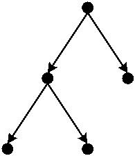
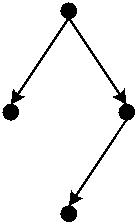


Combinatorial Algorithms: Let D = (V, A) and c : A → R+ be a non-negative cost function
on the the arcs. We wish to find a min-cost arborescence rooted at given node r ∈ V . We observe
that a greedy algorithm similar to Prim’s algorithm for computing an MST does not work.
r
3
4
1
v
u
For the above example, greedy method will pick (r, v) and then has to pick (r, u) for total cost
of 7. However, optimal arborescence is {(r, u), (u, v)} of cost 5.
Algorithm for min-cost r-aroborescence:
1. Let A0 = {a ∈ A | c(a) = 0} be the set of zero-cost arcs. If there is an r-arborescence in A0
(of cost 0), output it as the min-cost arborescence.
2
. Else, let S , . . . , S be the vertex sets of the strong connected components of D[A ]. Let
0
1
k
c(a), that is α is the cost of the min-cost edge entering S .
αi = mina∈δ
−1(Si)
i
i
for i = 1 to k do
for each a ∈ δ−1(Si)
c′(a) = c(a) − αi
3
. Recursively compute a min-cost arborescence in D = (V, A) with edge-cost function c′. Out-
put the solution of recursive call.
First, we argue that the algorithm terminates in polynomial time. If A0 does not contain an
r-arborescence then at least one Si has all incoming edges of strictly positive cost (why?) and hence
in step 2, at least one additional arc has its cost reduced to zero; thus the size of A0 increases and
hence at most O(m) recursive calls suffice. In fact, if we shrink each Si to a single vertex, one can
show that the number of vertices reduces by at least one and hence O(n) recursive calls suffice.
Since strong connected components can be found in O(m) time, this leads to an O(mn) running
time.
Now we argue correctness. It is easy to see that step 1 is correct. To argue correctness of step
3, we have the following lemma.
Lemma 3 Let S , . . . , S be vertex sets of the strong connected components of D[A ]. Then there
1
k
0
exists a min-cost arborescence A∗ in D s.t. |δ−1(S ) ∩ A | = 1.
∗
i
Proof: Say A is an optimal arborescence and |A ∩δ−1(Si)| ≥ 2. Let a = arg min
∗
∗
′
∗
c(a′)
a ∈A ∩δ−1(Si)
∗
′
∗
−1
′
be the least cost arc entering S in A . Then let A = (A \δ (S ))∪{a}∪(A ∩A[S ]); A is the set
i
i
0
i
∗
of arcs obtained by adding to A all zero-cost arcs inside S (A ∩A[S ]) and removing all arcs from
i
0
A that enter S other than the least cost arc a defined above. It is easy to check that A contains
i
∗
′
i
an r-arborescence and moreover its cost is no more than that of A0. Further, |δ−1(S ) ∩ A | = 1
′
i
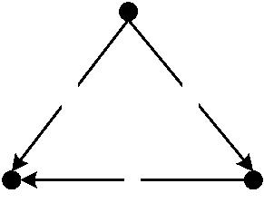
and |δ−1(S ) ∩ A | = |δ (S ) ∩ A | for all j = i. Repeating the above process for each S gives the
′
−1
∗
j
desired claim.
j
i
2
This leads to the following theorem.
Theorem 4 There is an O(nm) time algorithm to compute a min-cost r-arborescence in a directed
graph with n nodes and m edges.
There is an O(m + n log n)-time algorithm to find a min-cost r-arboresence problem which is
comparable to the standard MST algorithms.
Max-weight arborescences and Branchings. Since any arborescence has exactly n − 1 edges,
one can solve the max-weight arborescence by negating weights, adding a large positive number to
make weights positive and then computing a min-weight arborescence.
One can use the max-weight arborescence algorithm to compute a max- weight branching. Note
that given w : A → R, we can assume w(a) ≥ 0 ∀a by removing all arcs with negative weights.
We note that a max-weight branching may not be maximal even when weights are positive; this
is unlike the case of matroids (in particular, a max-weight forest is a spanning tree if all weights
are non-negative and the input graph is connected). To solve the max weight branching problem,
we add a new vertex r and connect it to each v ∈ V with an arc (r, v) of weight 0. Now we find a
max-weight arborescence rooted at r. We leave the correctness of this algorithm as an easy exercise.
2
.1 Polyhedral Aspects
One can obtain polyhedral descriptions for branchings and arborescences via matroid intersection.
However, some natural and direct descriptions exist.
Let Pr−arborescence(D) = convexhull{χ(B) | B is a r-arborescence in D}.
Theorem 5 Pr−arborescence(D) is determined by
x(a) ≥ 0 a ∈ A
x(δ−1(v)) = 1 v ∈ V \{r}
x(δ−1(U)) ≥ 1 U ⊆ V \{r}
Proof: We give an iterated rounding based proof to show that the following set of inequalities
0
≤ x(a) ≤ 1 a ∈ A
x(δ−1(U)) ≥ 1 U ⊆ V \{r}
is the convex hull of the characteristic vectors of arc sets that contain an r-arborescence. One can
easily adapt the proof to show the theorem statement. Let x be any basic feasible solution to the
above system. We claim that ∃a ∈ A s.t. x(a) = 0 or x(a) = 1. In either case, we obtain the
desired proof by induction on |A|. If x(a) = 0 we consider D[A \ {a}], if x(a) = 1, we shrink the
end points of a into a single vertex and consider the resulting graph.
We now prove that ∃a ∈ A s.t. x(a) ∈ {0, 1}. Assume not, then x(a) ∈ (0, 1) ∀a ∈ A. Let
F = {U ∈ V \{r} | x(δ−1(U)) = 1} be the collection of tight sets.
Claim 6 F is closed under intersections and unions.
Claim 7 Let L be a maximal laminar family in F. Then span({X(U) | U ∈ L})=span({X(U) |
U ∈ F}).
The above claims are based on uncrossing arguments that we have seen in several contexts. We
leave the formal proofs as an exercise.
Since L is a laminar family on V \{r}, we have
|L| ≤ 2(|V | − 1) − 1 ≤ 2|V | − 3
Since x(δ−1(v)) ≥ 1 for each v ∈ V \ {r} and x(a) ∈ (0, 1) for all a ∈ A,
δ−1(v) ∩ A| ≥ 2 ∀v ∈ V \ {r}
|
This implies that |A| ≥ 2|V | − 2. However, x is a basic feasible solution and L determines x, and
thus |L| = |A|, a contradiction.
2
In fact, one can show that the system of inequalities is TDI and this implies a min-max result
as well. See [1] for more details.
3
Arc-Disjoint Arborescences
A beautiful theorem of Edmonds is the following.
Theorem 8 Let D = (V, A) be a digraph and let r ∈ V . D has k arc-disjoint r-arborescences iff
for each v ∈ V \{r} there are k arc-disjoint paths from r to v.
Proof: If D has k arc-disjoint r-arborescences then clearly for each v ∈ V \{r}, there are k arc-
disjoint r → v paths in D, one in each of the arboresences.
We prove the converse via a proof given by Lov´asz using induction on k (proof adapted from
[2]). Let C = {U ⊂ V | r ∈ U} be the collection of all proper subsets of V that contain r. Note
that the condition that there are k-arc-disjoint paths from r to each v is equivalent to, by Menger’s
theorem,
|
δ+(U)| ≥ k ∀U ∈ C.
The idea is to start with the above condition and find an r-arborescence A1 s.t.
+
|
δ (U)\A | ≥ k − 1
∀U ∈ C.
1
Then, by induction, we will be done. We obtain A1 by growing an r-arborescence from r as follows.
We start with A1 = ∅ and S = {r}; S is the set of vertices reachable from r via arcs in the current
+
set of arcs A . We maintain the property that |δ (U)\A | ≥ k − 1 ∀U ⊂ S, r ∈ U. If we reach
1
S = V , we are done.
1
+
The goal is to find an arc in δ (S) to add to A and grow S. Call a set X ⊂ V critical/dangerous
1
if
•
•
•
X ∈ C and
X ∪ S = V and
+
|δ (X) \ A | = k − 1.
1
S
ꢀ
+(S)
Figure 1: S and δ+(S)
+
We observe that if there are no critical sets, any arc a ∈ δ (S) can be used to augment A . If
1
X is critical, then we cannot pick any unused arcs from δ (X) to grow A . The goal is to show
+
1
that there always exists an arc a ∈ δ+(S) such that a does not cross any critical set. We claim the
following uncrossing property for critical sets.
Claim 9 If X, Y are critical and X ∪ Y = V , then X ∩ Y and X ∪ Y are critical.
′
+
G′
Proof: Let G = G[A\A ], then |δ (X)| = k −1 and |δ (Y )| = k −1. We have, by submodularity
1
G′
+
G
of the cut function |δ ()|,
|
δ (X)| + |δ (Y )| ≥ |δ (X ∪ Y )| + |δ (X ∩ Y )|.
G′ G′ G′ G′
Since r ∈ X ∩ Y and r ∈ X ∪ Y and X ∪ Y = V , we have that |δG′ (X ∩ Y )| ≥ k − 1 and
|δG′ (X ∪ Y )| ≥ k − 1. Since X, Y are critical,
k − 1 + k − 1 ≥ |δ (X ∩ Y )| + |δ (X ∪ Y )| ⇒ δ (X ∩ Y ) = δ (X ∪ Y ) = k − 1.
G′
G′
G′
G′
2
Let X be a inclusion-wise maximal critical set.
Claim 10 There exists an arc (u, v) ∈ A s.t. u ∈ S \ X and v ∈ V \ (S ∪ X).
+
Proof: Note that A ∩ δ (S) = ∅ since S, by defintion, is a set of reachable nodes in A . Since
1
1
|
δ+(S ∪ X)| ≥ k (by assumption) and |δG+−A (X)| = k − 1 (since X is critical), we have an arc as
1
desired.
2
′
+
′
Now let A = A + (u, v). The claim is that for all U ∈ C, |δ (U) \ A | ≥ k − 1. Suppose not.
1
1
1
+
′
1
+
Then let Y be such that |δ (Y )\A | < k − 1 but this implies that |δ (Y )\A | = k − 1, that is Y is
1
S
r
X
+
Figure 2: All arcs from A ∩ δ (S) go from X to S
1
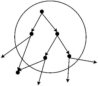
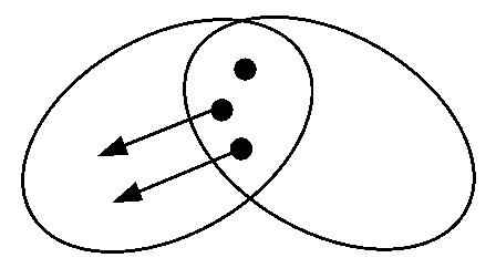
S
r
X
u
v
Figure 3: Claim 10
critical and (u, v) ∈ δ+(Y ). But consider Y , X both critical and Y ∪ X = V since v ∈/ Y , v ∈/ X.
Therefore X ∪ Y is critical, which contradicts maximality of X.
2
We note that the above theorem shows the integer decomposition property for the arboresence
polytope discussed earlier. The proof can be converted into a polynomial time algorithm to find
a maximum number of arc-disjoint r-arborescences in a given digraph. First we let k be the
minv∈V \{r} λ (r, v) where λ (r, v) is the arc-connectivity between r and v. The theorem guarantees
D
D
k r-aroboresences. In the above proof, the main issue is to find in each iteration an arc to augment
A with. We note that given an arc a, we can check if A + a satisfies the invariant by checking
1
1
′
the min-cut value from r to each node v, in the graph D = D[A \ (A + a)]. The proof guarantees
1
the existence of an arc a that can be used to augment A1 and hence one of the m arcs in D will
succeed. It is easy to see that this leads to a polynomial time algorithm. There is also a polynomial
time algorithm for the capacitated case. See [1] for details.
Edmonds derived the arc-disjoint r-arborescences theorem from a more general theorem on
disjoint branchings. We refer the reader to [1].
References
[1] A. Schrijver. Combinatorial Optimization. Springer-Verlag Berlin Heidelberg, 2003.
[2] B. Korte and J. Vygen. Combinatorial Optimization: Theory and Algorithms. Springer-Verlag,
Fourth Edition, 2008.
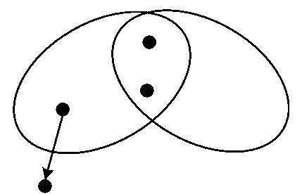
CS 598CSC: Approximation Algorithms
Instructor: Chandra Chekuri
Lecture date: April 22, 2009
Scribe: Zhenhui Li
We describe two well known theorems in combinatorial optimization. We prove the theorems
using submodular flows later.
1
Graph Orientation
Definition 1 Let G = (V, E) be an undirected graph. For u, v ∈ V , we denote by λG(u, v) the edge-
connectivity between u and v in G, that is, the maximum number of edge-disjoint paths between u
and v. Similarly for a directed graph D = (V, A), λD(u, v) is the maximum number of arc-disjoint
paths from u to v.
Note that for an undirected graph G, λ (u, v) = λ (v, u) but it may not be the case that
G
G
λ (u, v) = λ (v, u) in a directed graph D.
D D
Definition 2 G is k-edge-connected if λG(u, v) ≥ k ∀u, v ∈ V . Similarly, D is k-arc-connected if
λD(u, v) ≥ k ∀u, v ∈ V .
Proposition 1 G is k-edge-connected iff |δ(S)| ≥ k ∀S ⊂ V . D is k-arc-connected iff |δ+(S)| ≥ k
∀
S ⊂ V .
Proof: By Menger’s theorem.
2
Definition 3 D = (V, A) is an orientation of G = (V, E) if D is obtained from G by orienting
each edge uv ∈ E as an arc (u, v) or (v, u).
Theorem 2 (Robbins 1939) G can be oriented to obtain a strongly-connected directed graph iff
G is 2-edge-connected.
Proof: “⇒” Suppose D = (V, A) is a strongly connected graph obtained as an orientation of
G = (V, E). Then, since ∀S ⊂ V , |δ (S)| ≥
+
D
1 and δ (S)| ≥
D
| −
1, we have δ (S)| ≥ 2. Therefore, G
|
G
is 2-edge-connected.
“⇐” Let G be a 2-edge-connected graph. Then G has an ear-decomposition. In other words, G
is either a cycle C or G is obtained from a 2-edge-connected graph G′ by adding an ear P (a path)
connecting two not-necessarily distinct vertices u, v ∈ V .
G’
C
or
v
u
P
Figure 1: G is either a cycle C or is G′ plus an ear P.
If G = C, orient it to obtain a directed cycle which is strongly-connected. Otherwise, inductively,
G′ has an orientation that is strongly-connected. Extend the orientation of G′ to G by orienting

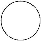
P from u to v (or v to u). It is easy to check that this orientation results in strongly-connected
graph.
2
An alternative proof is as follows. Do a depth-first-search (DFS) of G starting at some node r.
One obtains a DFS tree T. Orient all edges of T away from r to obtain an arborescence. Every
other edge is a back-edge, that is if uv ∈ E(G)\E(T), then, either u is the ancestor of v in T or v
is an ancestor of u in T. Orient uv from the descendant to the ancestor. We leave it as an exercise
to argue that this is a strongly-connected orientation of G iff G is 2-edge-connected. Note that this
is an easy linear time algorithm to obtain the orientation.
dashed edges are back edges
Figure 2: Orientation of a 2-edge-connected graph via a DFS tree.
Nash-Williams proved the following non-trivial extension.
Theorem 3 (Nash-Williams) If G is 2k-edge-connected, then it has an orientation that is k-
arc-connected.
In fact, he proved the following deep result, of which the above is a corollary.
Theorem 4 (Nash-Williams) G has an orientation D in which λ (u, v) ≥ ⌊λ (u, v)/2⌋ for all
D
G
u, v ∈ V .
The proof of the above theorem is difficult - see [1]. We will prove the easier version using
submodular flows later.
2
Directed Cuts and Lucchesi-Younger Theorem
Definition 4 Let D = (V, A) be a directed graph. We say that C ⊂ A is a directed cut if ∃S ⊂ V
such that δ+(S) = ∅ and C = δ−(S).
If D has a directed cut then D is not strongly-connected.
Definition 5 A dijoin (also called a directed cut cover) in D = (V, A) is a set of arcs in A that
intersect each directed cut of D.
It is not difficult to see that the following are equivalent:
•
B ⊆ A is a dijoin.
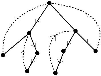
C
S
Figure 3: A directed cut C = δ−(S).
•
•
shrinking each arc in B results in a strongly-connected graph.
adding all reverse arcs of B to D results in a strongly-connected graph.
Given B ⊆ A, it is therefore, easy to check if B is a dijoin; simply add the reverse arcs of B to
D and check if the resulting digraph is strongly connected or not.
Definition 6 A digraph D is weakly-connected if the underlying undirected graph is connected.
Theorem 5 (Lucchesi-Younger) Let D = (V, A) be a weakly-connected digraph. Then the min-
imum size of a dijoin is equal to the maximum number of disjoint directed cuts.
A dijoin intersects every directed cut so its size is at least the the maximum number of disjoint
directe cuts. The above theorem is yet another example of a min-max result. We will prove this
later using submodular flows. One can derive easily a weighted version of the theorem.
Corollary 6 Let D = (V, A) be a digraph with ℓ : A → Z+. Then the minimum length of a dijoin
is equal to the maximum number of directed cuts such that each arc a is in at most ℓ(a) of them
(in other words a maximum packing of directed cuts in ℓ).
Proof: If ℓ(a) = 0, contract it. Otherwise replace a by a path of length ℓ(a). Now apply the
Lucchesi-Younger theorem to the modified graph.
2
As one expects, a min-max result also leads to a polynomial time algorithm to compute a
minimum weight dijoin and a maximum packing of directed cuts.
Woodall conjectured the following, which is still open. Some special cases have been solved [1].
Conjecture 1 (Woodall) For every directed graph, the minimum size of a directed cut equals to
the maximum number of disjoint dijoins.
We describe an implication of Lucchesi-Younger theorem.
Definition 7 Given a directed graph D = (V, A), A′ ⊆ A is called a feedback arc set if D[A \ A′]
is acyclic, that is, A′ intersects each directed cycle of D.
Computing a minimum cardinality feedback arc set is NP-hard. Now suppose D is a plane
directed graph (i.e., a directed graph that is embedded in the plane). Then one defines its dual
graph D∗ as follows. For each arc (w, x) of D, we have a dual arc (y, z) ∈ D∗ that crosses (w, x)
from “left” to “right”. See example below.
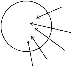
Figure 4: A planar digraph and its dual.
Proposition 7 The directed cycles of D correspond to directed cuts in D∗ and vice versa.
Thus, a feedback arc set of D corresponds to a dijoin in D∗. Via Lucchesi-Younger theorem,
we have the following corollary.
Corollary 8 For a planar directed graph, the minimum size of a feedback arc set is equal to the
maximum number of arc-disjoint directed cycles.
Using the algorithm to compute a minimum weight dijoin, we can compute a minimum weight
feedback arc set of a planar digraph in polynomial time.
3
Polymatroid Intersection
Recall the definition of total dual integrality of a system of inequalities.
Definition 8 A rational system of inequalities Ax ≤ b is TDI if for all integral c, min{yb | y ≥
0, yA = c} is attained by an integral vector y∗ whenever the optimum exists and is finite.
Definition 9 A rational system of inequalities Ax ≤ b is box-TDI if the system d ≤ x ≤ c, Ax ≤ b
is TDI for each d, c ∈ Rn.
In particular, we have the following. If Ax ≤ b is box-TDI, then the polyhedron {x | Ax ≤
b, d ≤ ℓ ≤ u} is an integer polyhedron whenever b, ℓ, u are integer vectors.
Recall that if f : 2S → R is a submodular function, EPf is the extended polymatroid defined
as
{
x ∈ RS|x(U) ≤ f(U), U ⊆ S}
We showed that the system of inequalities x(U) ≤ f(U), U ⊆ S is TDI. In fact, one can
show that the system is also box-TDI. Polymatroids generalize matroids. One can also consider
polymatroid intersection which generalizes matroid intersection.
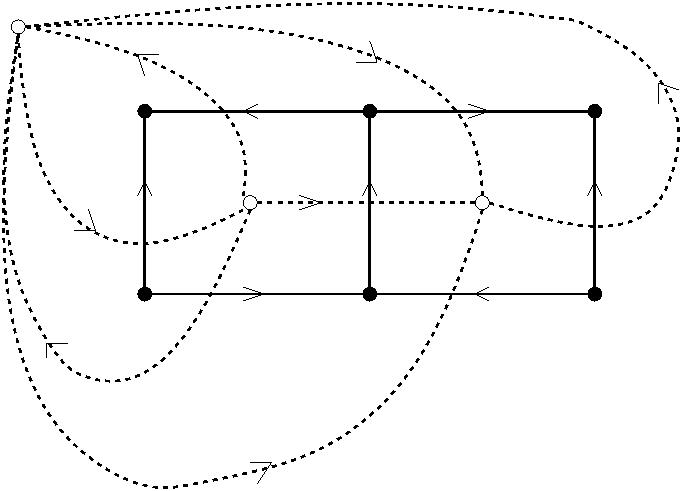
Let f , f be two submodular functions on S. Then the polyhedron EP ∩ EPf2 described by
1
2
f1
x(U) ≤ f1(U)
x(U) ≤ f2(U)
U ⊆ S
U ⊆ S
is an integer polyhedron whenever f and f are integer valued. We sketch a proof of the following
1
2
theorem.
Theorem 9 (Edmonds) Let f , f be two submodular set functions on the ground set S. The
1
2
system of inequalities
x(U) ≤ f1(U)
x(U) ≤ f2(U)
U ⊆ S
U ⊆ S
is box-TDI.
Proof: (Sketch) The proof is similar to that of matroid intersection. Consider primal-dual pair
below
max wx
x(U) ≤ f1(U)
x(U) ≤ f2(U)
U ⊆ S
U ⊆ S
ℓ ≤ x ≤ u
P
P
P
min
(f (U)y (U) + f (U)y (U)) +
U⊆S P1
u(a)z1(a) −
ℓ(a)z2(a)
a∈S
1
2
2
a∈S
(y (U) + y (U)) + z (a) − z (a) = w(a), a ∈ S
a∈U
1
2
1
2
y ≥ 0, z , z ≥ 0
1
2
Claim 10 There exists an optimal dual solution such that F = {U | y (U) > 0} and F = {U |
1
1
2
y2(U) > 0} are chains.
The proof of the above claim is similar to that in matroid intersection. Consider F1 = {U |
y (U) > 0}. If it is not a chain, there exist A, B ∈ F such that A ⊂ B and B ⊂ A. We change
1
1
y by adding ǫ to y (A ∪ B) and y (A ∩ B) and subtracting ǫ from y (A) and y (B). One observes
1
1
1
1
1
that the feasibility of the solution is maintained and that the objective function can only decrease
since f is submodular. Thus, we can uncross repeatedly to ensure that F is a chain, similarly F .
1
1
2
Let y , y , z , z be an optimal dual solution such that F and F are chains. Consider F = F ∪
1
2
1
2
1
2
1
F2 and the S ×F incidence matrix M. As we saw earlier in the proof for matroid intersection, M is
TUM. We then have y , y , z , z are determined by a system [ y y2 z1 z2 ][ M −I ] = w,
−I ] is TUM, there exists integer optimum
I
1
2
1
2
1
where w is integer and M is TUM. Since [ M
I
solution.
2
Note that, one can separate over EP ∩EP via submodular function minimization and hence
f
f2
1
one can optimize EPf1 ∩ EPf2 in polynomial time via the ellipsoid method. Strongly polynomial
time algorithm can also be derived. See [1] for details.
4
Submodularity on Restricted Families of Sets
So far we have seen submodular functions on a ground set S. That is f : 2S → R and ∀A, B ⊆ S,
f(A) + f(B) ≥ f(A ∩ B) + f(A ∪ B)
In several applications, one needs to work with restricted families of subsets. Given a finite set
S, a family of sets C ⊆ 2S is
•
•
•
a lattice family if ∀A, B ∈ C, A ∩ B ∈ C and A ∪ B ∈ C.
an intersecting family if ∀A, B ∈ C and A ∩ B = ∅, we have A ∩ B ∈ C and A ∪ B ∈ C.
a crossing family if A, B ∈ C and A∩B = ∅ and A∪B = S, we have A∩B ∈ C and A∪B ∈ C.
For each of the above families, a function f is submodular on the family if
f(A) + f(B) ≥ f(A ∪ B) + f(A ∩ B)
whenever A ∩ B, A ∪ B are guaranteed to be in family for A, B. Function f is called intersection
submodular and crossing submodular if C is intersecting and crossing family respectively.
We give some examples of interesting families that arise from directed graphs. Let D = (V, A)
be a directed graph.
Example 1 C = 2V \ {∅, V } is a crossing family.
Example 2 Fix s, t ∈ V , C = {U | s ∈ U, t ∈/ U} is lattice, intersecting, and crossing family.
Example 3 C = {U ⊂ V | U induces a directed cut i.e. δ+(U) = ∅ and ∅ ⊂ U ⊂ V } is a crossing
family.
For the above example, we sketch the proof that C is a crossing family. If A, B ∈ C and A∩B = ∅
and A ∪ B = V , then by submodularity of δ+, |δ+(A ∪ B)| + |δ+(A ∩ B)| ≤ |δ+(A)| + |δ+(B)|.
Therefore we have δ+(A∪B) = ∅ and δ+(A∩B) = ∅ and more over A∩B and A∪B are non-empty.
Hence they both belong to C as desired.
Various polyhedra associates with submodular functions and the above special families are
known to be well-behaved.
For lattice families the system
x(U) ≤ f(U), U ∈ C
is box-TDI. Also, the following system is also box-TDI
x(U) ≤ f1(U), U ∈ C1
x(U) ≤ f2(U), U ∈ C2
where C and C are lattice families and f and f are submodular on C and C2 respectively. The
1
2
1
2
∞
above facts also hold for intersecting families and intersecting submodular functions.
For crossing family C, the system
x(U) ≤ f(U)
is not necessarily TDI. However, the system
x(U) ≤ f(U), U ∈ C
x(S) = k
where k ∈ R is box-TDI. Also, the system
x(U) ≤ f1(U), U ∈ C1
x(U) ≤ f2(U), U ∈ C2
x(S) = k
is box-TDI for crossing families C and C with f and f crossing supermodular on C and C
2
1
2
1
2
1
respectively.
Although the polyhedra are well-behaved, the separation problem for them is not easy since
one needs to solve submodular function minimization over a restricted family C. It does not suffice
to have a value oracle for f on sets in C; one needs additional information on the representation of
C. We refer the reader to [1] for more details.
References
[1] A. Schrijver. Combinatorial Optimization. Springer-Verlag Berlin Heidelberg, 2003.
[2] Lecture notes from Michel Goemans’s class on Combinatorial Optimization. http://www-
math.mit.edu/ goemans/18997-CO/co-lec18.ps
CS 598CSC: Combinatorial Optimization
Instructor: Chandra Chekuri
Lecture date: April 27th, 2010
Scribe: Peixiang Zhao
1
Submodular Flows
Network flows are a fundamental object and tool in combinatorial optimization. We have also seen
submodular functions and their role in matroids, matroid intersection, polymatroids and polyma-
troid intersection. Edmonds and Giles developed the framework of submodular flows to find a
common generalization of network flow and polymatroid intersection. Here is the model.
Definition 1 (Crossing Family) Let D = (V, A) be a directed graph and let C ⊆ 2V be a family
of subsets of V. C is called a crossing family if: A, B ∈ C , A ∩ B = ∅, A ∪ B = V ⇒ A ∩ B ∈ C
and A ∪ B ∈ C .
Definition 2 (Crossing Submodular) Let C be a crossing family. A function f : C → R is
called crossing submodular on C if it satisfies: A, B ∈ C , A∩B = ∅, A∪B = V ⇒ f(A)+f(B) ≥
f(A ∪ B) + f(A ∩ B).
Definition 3 (Submodular Flow) Let D = (V, A) be a digraph, C be a crossing family, and f
be a crossing submodular function on C . A vector x ∈ RA is called a submodular flow if
x(δ−(u)) − x(δ+(u)) ≤ f(u),
∀u ∈ C
(1)
Theorem 4 (Edmonds-Giles, 1977) The system of inequalities shown in Equation 1 is box-TDI
where C is a crossing family on V and f is crossing submodular on C .
Proof: We consider the primal-dual pair of LPs below where w : A → Z+ and ℓ, u are integer
vectors.
X
max
wx
s.t.
x(δ−(U)) − x(δ+(U)) ≤ f(U)
ℓ ≤ x ≤ u
U ∈ C
and
X
X
X
min
f(U)y(U) +
u(a)z1(a) −
ℓ(a)z2(a)
U∈C
a∈A
a∈A
X
X
s.t.
y(U) −
y(U) + z (a) − z (a) = w(a)
a ∈ A
1
2
U:U∈C ,a∈δ−(U)
U:U∈C,a∈δ+(U)
y, z , z ≥ 0
1
2
A family of sets F ⊆ 2V is cross-free if for all A, B ∈ F the following holds:
A ⊆ B or B ⊆ A or A ∩ B = ∅ or A ∪ B = V .

Claim 5 There exists an optimum solution y, z , z such that F = {U ∈ C | y(U) > 0} is cross-
1
2
free.
Proof: Suppose F is not cross-free. Then let A, B ∈ F, such that y(A) > 0 and y(B) > 0 and
A ∩ B = ∅ and A ∪ B = V . Then add ǫ > 0 to y(A ∪ B), y(A ∩ B) and subtract ǫ > 0 from y(A)
and y(B). By submodularity of f, the objective function increases or remains same. We claim that
alterting y in this fashion maintains dual feasibility; we leave this as an exercise.
By repeated uncrossing we can make F cross-free. Formally one needs to consider a potential
function. For example, among all optimal solutions pick one that minimizes
X
y(U)|U||V \U|
U∈C
2
Theorem 6 Let F be a cross-free family on 2V . Let M be an |A| × |F| matrix where
if a δ−(U)
−1 if a ∈ δ+(U)
otherwise
∈
1
Ma,U
=
0
Then M is TUM.
The proof of the above theorem proceeds by showing that M is a network matrix. See Schrijver
Theorem 13.21 for details [1].
By the above one sees that the non-negative components of y, z , z are determined by [M, I, −I]
1
and integer vector w where M is TUM. From this we infers that there exists an integer optimum
2
solution to the dual.
2
Corollary 7 The polyhedron P determined by
x(δ−(U)) − x(δ+(U)) ≤ f(U)
U ∈ C
l ≤ x ≤ u
is an integer polyhedron whenever f is integer valued and l, u are integer vectors.
One can show that optimality on P can be done in strongly polynomial time if one has a value
oracle for f. This can be done via a reduction to polymatroid intersection. We refer to Schrijver,
Chapter 60 for more details [1].
2
Applications
Submodular flows are a very general framework as they combine graphs and submodular functions.
We gave several applications below.
2
.1 Circulations
Given a directed graph D = (V, A), x : A → R is a circulation if
x(δ−(v)) − x(δ+(v)) = 0,
∀v ∈ V
This can be modeled as a special case of submodular flow by setting C = {{v} | v ∈ V } and f = 0.
We get the inequalities
x(δ−(v)) − x(δ+(v)) ≤ 0,
v ∈ V.
One can check that the above inequalities imply that for any ∅ ⊂ U ⊂ V the inequality x(δ−(U) −
x(δ+(U) ≤ 0 holds by adding up the inequalities for each v ∈ U. Combining this with the inequality
x(δ−(V \U)−x(δ (V \U) ≤ 0, we have x(δ (U)−x(δ (U) = 0 for all ∅ ⊂ U ⊂ V and in particular
+
−
+
for each v ∈ V . The box-TDI result of submodular flow implies the basic results on circulations
and flows including Hoffman’s circulation theorem and the max-flow min-cut theorem.
2
.2 Polymatroid Intersection
We saw earlier that the system
x(U) ≤ f1(U)
x(U) ≤ f2(U)
U ⊆ S
U ⊆ S
is box-TDI whenever f , f are submodular functions on S. We can derive this from submodular
1
2
U
flows as follows. Define S′ and S′′ are copies of S. Let V = S′ S′′ and define C = {U′ | U ⊆
S} ∪ {S′ ∪ U′′ | U ⊆ S}, where U′ and U′′ denote the sets of copies of elements of U in S′ and
S′′ [1].
Claim 8 C is a crossing family.
Exercise 9 Prove Claim 8.
We further define f : C → R+ by
f(U′) = f1(U)
U ⊆ S
U ⊆ S
f(V \U′′) = f2(U)
f(S′) = min{f (S), f (S)}
1
2
Claim 10 f is crossing submodular on C .
Exercise 11 Prove Claim 10.
Now define G = (V, A) where A = {(s′′, s′)|s ∈ S}, as shown in Figure 1. The submodular flow
polyhedron is
x(δ−(Z)) − x(δ+(Z)) ≤ f(Z)
Z ∈ C
If Z = U′ where U ⊆ S, then we get x(U) ≤ f1(U). And if Z = V \U′′, as shown in Figure 2, then
we get x(U) ≤ f2(U), U ⊆ S. Thus, we recover the polymatroid intersection constraints. Since the
submodular flow constraint inequalities are box-TDI, it implies that the polymatroid intersection
constraints are also box-TDI.
Figure 1: A Directed Graph Defined on S
Figure 2: Z = V \U′′
2
.3 Nash-Williams Graph Orientation Theorem
We stated the following theorem of Nas-Williams in the previous lecture.
Theorem 12 If G is 2k-edge-connected then it has an orientation D such that D is k-arc-connected.
Frank(1980) [2] showed that Theorem 12 can be derived from submodular flows. Consider an
arbitrary orientation D of G. Now if D is k-arc-connected we are done. Otherwise we consider
the problem of reversing the orientation of some arcs of D such that the resulting graph is k-arc-
connected. We set it up as follows.
Let D = (V, A), define a variable x(a), a ∈ A where x(a) = 1 if we reverse the orientation of
a. Otherwise x(a) = 0. For a set U ⊂ V we want k arcs coming in after applying the switch of
orientation, i.e., we want
x(δ−(u)) − x(δ (u)) ≤ |δ (u)| − k
+
−
∀ ∅ ⊂ U ⊂ V
Note that C = {U | ∅ ⊂ U ⊂ V } is a crossing family and f(U) = |δD−(u)|−k is crossing submodular.
Hence by Edmonds-Giles theorem, the polyhedron determined by the inequalities
x(δ−(u)) − x(δ (u)) ≤ |δ (u)| − k
+
−
∅ ⊂ U ⊂ V
x(a) ∈ [0, 1] a ∈ A
is an integer polyhedron. Moreover, the polyhedron is non-empty since x(a) = 1/2, ∀a ∈ A satisfies
all the constraints. To see this, let ∅ ⊂ U ⊂ V , and let h = δ−(U) and ℓ = δ (U), then we have
+
D
D
h + ℓ ≥ 2k since G is 2k-edge-connected. Then by setting x(a) = 1/2, ∀a ∈ A, for U we need
h
l
h + l
−
≤ h − k ⇒
≤ k
2
2
2
which is true. Thus there is an integer vector x in the polyhedron for D if G is 2k-edge-connected.
By reversing the arcs A′ = {a|x(a) = 1} in D we obtain a k-arc-connected orientation of G.
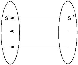


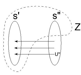


2
.4 Lucchesi-Younger theorem
Theorem 13 (Lucchesi-Younger) In any weakly-connected digraph, The size of the minimum
cardinality dijoin equals the maximum number of disjoint directed cuts.
Proof: Let D = (V, A) be a directed graph and let C = {U | ∅ ⊂ U ⊂ V, |δ+(U)| = 0}, i.e.,
U ∈ C iff U induces a directed cut. We had seen that C is a crossing family. Let f : C → R
be f(U) = −1, ∀U ∈ C , clearly f is crossing submodular. Then by Edmonds-Giles theorem the
following set of inequalities is TDI.
x(δ−(U)) − x(δ+(U)) ≤ −1
x ≤ 0
U ∈ C
We note that δ+(U) = ∅ for each U ∈ C . We can rewrite the above polyhedron as the one below
by replacing −x by x.
x(δ−(U)) ≥ 1
x ≥ 0
U ∈ C
Note that the above is a “natural” LP relaxation for finding a set of arcs that cover all directed
cuts. The above polyhedron is integral, and hence
X
min
x(a)
a∈A
x(δ−(U)) ≥ 1
x ≥ 0
U ∈ C
gives the size of a minimum cardinality dijoin.
Consider the dual
max
X
y(U)
U∈C
X
s.t.
y(U) ≤ 1
a ∈ A
U:a∈δ−(U),U∈C
y ≥ 0
The dual is an integer polyhedron since the primal inequality system is TDI and the objective
function is an integer vector. It is easy to see that the optimum value of the dual is a maximum
packing of arc-disjoint directed cuts. Therefore by strong duality we obtain the Lucchesi-Younger
theorem.
2
References
[1] Lex Schrijver, “Combinatorial Optimization: Polyhedra and Efficiency, Vol. B”, Springer-
Verlag, 2003.
[2] Lecture notes from Michael Goemans’s class on Combinatorial Optimization, http://www-
math.mit.edu/~goemans/18997-CO/co-lec18.ps, 2004.
CS 598CSC: Combinatorial Optimization
Instructor: Chandra Chekuri
Lecture date: April 29, 2010
Scribe: Lu Su
1
Multiflows
The maxflow-mincut theorem of Ford and Fulkerson generalizes Menger’s theorem and is a funda-
mental result in combinatorial optimization with many applications.
Theorem 1 In a digraph D = (V, A) with arc capacity function c : A → R+, the maximum s-t
flow value is equal to the minimum s-t capacity cut value. Moreover, if c is integer valued, then
there is an integer valued maximum flow.
In particular, the maximum number of s-t arc-disjoint paths in a digraph is equal to the min-
imum number of arcs whose removal disconnects s from t (Menger’s theorem). When applied to
undirected graphs we obtain the edge-disjoint and node-disjoint path version of Menger’s Thoerem.
In many applications in networks we are interested in multiflows, also referred to as multi-
commodity flows. s − t flows are also referred to as single-commodity flows.
A multiflow instance in a directed graph consists of a directed “supply” graph D = (V, A)
with non-negative arc capacities c : A → R+ and a demand graph H = (T, R) with T ⊆ V called
terminals, and non-negative demand requirements d : R → R+. The arcs in R are referred to as
nets. The demand graph can also be specified as a set of ordered pairs (s , t ), . . . , (s , t ) with
1
1
k
k
di ∈ R+ denoting the demand for (s , t ). This is referred to as the k-commodity flow problem.
i
i
A multiflow instance in an undirected graph consists of an undirected supply graph G = (V, E)
and an undirected demand graph H = (T, R). The demand graph can be specified by a collection
of unordered pairs s t , . . . , s t .
1
1
k k
Given a multiflow instance in a directed graph D = (V, A) with demand graph H = (T, R), a
multiflow is a collection of flows, f , r ∈ R where f is an s -t flow and r = (s , t ). A multiflow
r
r
r
r
satisfies the capacity constraints of the supply graph if for each arc a ∈ A,
r
r
X
fr(a) ≤ c(a).
(1)
r∈R
The multiflow satisfies the demands if for each r = (s , t ) ∈ R, the f flow from s to t is at
r
r
r
r
r
least d(r).
For undirected graphs we need a bit more care. We say that f : E → R+ is an s − t flow if
there is an orientation D = (V, A) of G = (V, E) such that f′ : A → R+ defined by the orientation
and f : E → R+ is an s − t flow in D. Thus f , r ∈ R where f : E → R is a multiflow if each fr
r
r
+
is an s -t flow. It satisfies the capacity constraints if ∀e ∈ E,
r
r
X
fr(e) ≤ c(e).
(2)
r∈R
We say a multiflow is integral if each of the flows is integer valued; that is fr(a) is an integer for
each arc a and each r ∈ R. Similarly half-integral (i.e., each flow on an arc is an integer multiple
of 1/2).

Proposition 2 Given a multiflow instance in a directed graph, there is a polynomial time algorithm
to check if there exists a multiflow that satisfies the capacities of the supply graph and the demand
requirements of the demand graph.
Proof: Can be solved by expressing the problem as a linear program. Variables fr(a) r ∈ R, a ∈ A.
Write standard flow conservation constraints that ensures fr : A → R+ is a flow for each r (flow
conservation at each node other than the source and destination of r). We add the following set of
constraints to ensure capacity constraints of the supply graph are respected.
X
fr(a) ≤ c(a) a ∈ A.
(3)
r∈R
Finally, we add constraints that the value of fr (leaving the source of r) should be at least d(r). 2
Proposition 3 Given an undirected multiflow instance, there is a polynomial time algorithm to
check if there is a feasible multiflow that satisfies the supply graph capacities and the demand
requirements.
Proof: We reduce it to the directed flow case as follows. Given G = (V, E) obtain a digraph D =
−→ ←−
(V, A) by dividing each edge e into two arcs e and e . Now we have variable f (a), a ∈ A, r ∈ R,
r
and write constraints that ensure that fr : A → R+ is a flow of value d(r) from s to t where
r
r
r = s t . The capacity constraint ensures that the total flow on both e and e is at most c(e), i.e.,
−→
←−
r r
X
−→
←−
(f ( e ) + f ( e )) ≤ c(e), e ∈ E.
r
(4)
r
r∈R
2
LP duality gives the following useful necessary and sufficient condition; it is some times referred
to as the Japanese theorem.
Theorem 4 A multiflow instance in directed graph is feasible iff
X
k
X
d ℓ(s , t ) ≤
i
c(a)ℓ(a)
(5)
i
i
i=1
a∈A
for all length functions ℓ : A → R+.
Here ℓ(s , t ) is the shortest path distance from s to t with arc lengths ℓ(a). For undirected
i
i
graph the characterization is similar
i
i
X
k
X
d ℓ(s , t ) ≤
i
c(e)ℓ(e)
(6)
i
i
i=1
e∈E
for all ℓ : E → R+.
Proof: Consider the path formulation we prove it for undirected graphs. Let Pi be the set of s t
i i
path in G. Let f : P → R be an assignment of flow values to paths in Pi. We want feasibility of
i
i
+
X
fi(p) ≥ di i = 1 to k
(7)
p∈Pi
X
k
X
fi(p) ≤ c(e) e ∈ E
(8)
(9)
i=1 p∈Pi:e∈p
fi(p) ≥ 0, p ∈ Pi, 1 ≤ i ≤ k.
We apply Farkas lemma. Recal that Ax ≤ b, x ≥ 0 has a solution iff yb ≥ 0 for each row vector
y ≥ 0 with yA ≥ 0. We leave it as an exercise to derive the statement from Farkas lemma applied
to the above system of inequalities.
2
It is useful to interpret the necessity of the condition. Suppose for some ℓ : E → R+
X
k
X
d l(s , t ) >
i
c(e)ℓ(e)
(10)
i
i
i=1
e∈E
we show that there is no feasible multiflow. For simplicity assume ℓ is integer valued. Then
replace an edge e with length ℓ(e) by a path of length ℓ(e)
and place capacity c(e) on each edge. Suppose there is a feasible flow. For each (s , t ), each
i
flow path length is of length at least l(s , t ) ⇒ total capacity used up by flow for (s , t ) is ≥
i
P
P
k
i
i
i
i
d ℓ(s , t ). But total capacity available is
P
e∈E
c(e)ℓ(e) (after expansion). Hence if
d ℓ(s , t ) >
i=1
i
i
i
c(e)ℓ(e), there cannot be a feasible multiflow.
i
i
i
e
To show that a multiflow instance is not feasible it is sufficient to give an appropriate arc length
function that violates the necessary condition above.
2
Integer Multiflow and Disjoint Paths
When all capacities are 1 and all demands are 1 the problem of checking if there exists an inte-
ger multiflow is the same as asking if there exist arc-disjoint path (edge-disjoint path if graph is
undirected) connecting the demand pairs.
The edge-disjoint paths problem (EDP) is the following decision problem: given supply graph
D = (V, A) (or G = (V, E)) and a demand graph H = (T, R), are there arc/edge-disjoint paths
connecting the pairs in R?
Theorem 5 (Fortune-Hopcroft-Wyllie 1980) EDP in directed graphs is NP-complete even for
two pairs.
Theorem 6 EDP in undirected graphs is NP-complete when |R| is part of the input, even when
|R| consists of three sets of parallel edges.
A deep, difficult and fundamental result of Robertson and Seymour is that EDP in undirected
graphs is polynomial-time solvable when |R| is fixed. In fact they prove that the vertex-disjoint
path problem (the pairs need to be connected by vertex disjoint paths) is also tractable.
Theorem 7 (Robertson-Seymour) The vertex-disjoint path problem is polynomial-time solvable
if the number of demand pairs is a fixed constant.
The above theorem relies on the work of Robertson and Seymour on graph minors.

3
Cut Condition—Sparsest Cuts and Flow-Cut Gaps
A necessary condition for the existence of a feasible multiflow for a given instance is the so called
cut-condition. In directed graphs it is
+
D
+
H
c(δ (U)) ≥ d(δ (U)) ∀U ⊂ V
(11)
u
Demand arcs
Supply arcs
+
+
where c(δ (U)) is capacity of all arcs leaving U, and d(δ (U)) is the demand of all demand arcs
H
D
leaving U. It is easy to see that this condition is necessary. Formally one sees that this condition is
+
D
necessary by considering the length function ℓ : A → R where ℓ(a) = 1 if a ∈ δ (U) and ℓ(a) = 0.
+
For undirected graphs the cut condition states
+
G
+
H
c(δ (U)) ≥ d(δ (U)) ∀U ⊂ V
(12)
u
Demand arcs
Supply arcs
Cut condition is not sufficient in general. Consider the following examples in directed graphs
s1
S2
t1
s1
t2
S2
t1
t2
Cut condition is true for each case but no feasible multiflows exists as can be seen by considering
the length function ℓ(a) = 1 for each arc a.
For undirected graphs the following example is well known. Supply graph is K2,3, a series-
parallel graph. Again, cut-condition is satisfied but ℓ(e) = 1 for each e shows no feasible multiflow
exists.
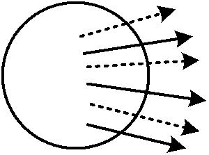
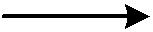
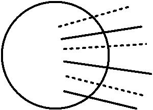


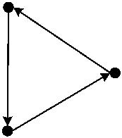
Dotted edges are
demand edges
4
Sufficiency of Cut Condition
Given that the cut condition is not sufficient for feasible flow it is natural to consider cases
where it is indeed sufficient. First consider directed graphs. Suppose we have demand pairs
of the form (s, t ), (s, t ), . . . , (s, t ), i.e., all pairs share a common source. Then it is easy to
1
2
k
see that cut condition implies feasible multiflow by reduction to the single-commodity flow case
by connecting t , t , . . . , t to a common sink t. Similarly if the demand pairs are of the form
1
2
k
(s , t), (s , t), . . . , (s , t) with a common source.
1
2
k
It turns out that these are the only interesting cases for which cut condition suffices. See
Theorem 70.3 in Schrijver Book.
For undirected graphs several non-trivial and interesting cases where the cut-condition is suffi-
cient are known. We list a few below:
•
•
Hu’s 2-commodity theorem shows that if there are only two pairs s t and s t then cut-
2 2
1
1
condition is sufficient.
Okamura-Seymour theorem states that if G is a planar graph and T is vertex set of a single
face then cut condition is sufficient. Note that the theorem implies that for capacitated ring
supply graphs the cut condition is sufficient.
•
•
Okamura’s theorem generalizes Okamura-Seymour Theorem. If G is planar and there are two
faces F and F such that each st ∈ R has both s, t on one of the faces then cut condition is
sufficient.
1
2
Seymour’s Theorem shows that if G + H is planar then cut condition is sufficient.
For all of the above cases one has the following stronger result. If G + H is Eulerian then
the flow is guaranteed to be integral. To see that the Eulerian condition is necessary for integral
flow in each of the above cases, consider the example below where the only feasible multiflow is a
half-integral.
t2
t1
s1
Only ½ integral
flow exists
s2
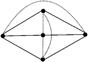
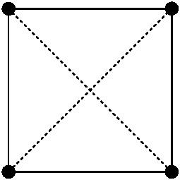
CS 598CSC: Combinatorial Optimization
Instructor: Chandra Chekuri
Lecture date: May 4th, 2010
Scribe: Dong Ye
1
Okamura-Seymour Theorem
Theorem 1 Let G = (V, E) be a plane graph and let H = (T, R) be a demand graph where T is
the set of vertices of a single face of G. Then if G satisfies the cut condition for H and G + H is
eulerian, there is an integral multiflow for H in G.
The proof is via induction on 2|E| − |R|. Note that if G satisfies the cut condition for H, then
|
R| ≤ |E| (why?).
There are several “standard” induction steps and observations that are used in this and other
proofs and we go over them one by one. For this purpose we assume G, H satisfy the conditions
of the theorem and is a counter example with 2|E(G)| − |R| minimal[1].
Claim 2 No demand edge r is parallel to a supply edge e.
Proof: If r is parallel to e then G−e, H −r satisfy the conditions of the theorem and by induction
H − r has an integral multiflow in G − e. We can route r via e. Thus H has an integral multiflow
in G.
2
Definition 3 A set S ⊂ V is said to be tight if |δ (S)| = |δ (S)|.
G
H
Claim 4 For every demand edge r ∈ R there is a tight cut S s.t. r ∈ δH(S).
Proof: If r is not in any tight set, then adding two copies of r to H maintains cut condition and
the Eulerian condition. By induction (note that the induction is on 2|E| − |R|) the new instance is
routable.
2
Claim 5 G is 2-node connected.
Proof: Suppose not and let v be a cut vertex of G. Let G , G , ..., G be the graphs obtained by
1
2
k
combining v with the components of G − v.
Suppose there is a demand edge r = (s, t) s.t. s = v, t = v and s ∈ G and t ∈ G , i = j. Then we
i
j
can replace (s, t) by two edges (s, v) and (v, t). The claim is that this new instance satisfies the cut
condition - we leave the formal proof as an exercise. Clearly Euler condition is maintained. The
new instance is routable by induction which implies that the original instance is also routable.

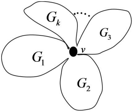
If no such demand edge exits then all demand edges have both end points in Gi for some i.
Then let H be the demand graph induced on G . We can verify that each G , H satisfy the cut
i
i
i
i
condition and the Euler condition. By induction each H is routable in G which implies that H is
i
i
routable in G.
2
Definition 6 A set ∅ ⊂ S ⊂ V is central if G[S] and G[V \ S] are connected.
Lemma 7 Let G be a connected graph. Then G, H satisfy the cut condition if and only if the cut
condition is satisfied for each central set S.
Proof: Clearly, if G, H satisfy the cut condition for all sets then it is satisfied for the central sets.
Suppose the cut condition is satisfied for all central sets but there is some non-central set S0 such
that |δ (S)| < |δ (S)|. Choose S0 to be minimal among all such sets. We obtain a contradiction
G
H
as follows. Let S , S , . . . , S be the connected components in G \ δ (S0); since S0 is not central,
1
2
k
G
k ≥ 3. Moreover each S is completely contained in S
0
or in
V \ S
0. We claim that some
S
j
violates
i
the cut-condition, whose proof we leave as an exercise. Moreover, by minimality in the choice of
S S
,
0
is central, contradicting the assumption.
2
j
One can prove the following corollary by a similar argument.
Corollary 8 Let G, H satisfy the cut condition. If S0 is a tight set and S0 is not central, then there
is some connected component S contained in S0 or in V \ S0 such that S is a tight central set.
Uncrossing:
Lemma 9 Let G, H satisfy cut-condition, Let A, B be two tight sets such that A ∩ B = ∅ and
A ∪ B = V . If |δ (A)| + |δ (B)| ≤ |δ (A ∩ B)| + |δ (A ∪ B)|, then A ∩ B and A ∪ B are tight. If
H
H
H
H
|
δ (A)| + |δ (B)| ≤ |δ (A − B)| + |δ (B − A)|, then A − B and A − B are tight.
H
H
H
H
Proof: By submodularity and symmetry of the cut function |δ | : 2V → R , we have
G
+
|
δ (A)| + |δ (B)| ≥ |δ (A ∩ B)| + |δ (A ∪ B)|
G
G
G
G
and also
δ (A)| + |δ (B)| ≥ |δ (A − B)| + |δ (B − A)|.
G
G
G
G
Now if
|
δ (A)| + |δ (B)| ≤ |δ (A ∩ B)| + |δ (A ∪ B)|
H
H
H
H
then we have
|
δ (A ∩ B)| + |δ (A ∪ B)| ≥ |δ (A ∩ B)| + |δ (A ∪ B)| ≥ |δ (A)| + |δ (B)| = |δ (A)| + |δ (B)|
G
G
H
H
H
H
G
G
where the first inequality follows from the cut-condition, the second from our assumption and the
third from the tightness of A and B. It follows that
|
δ (A ∩ B)| = |δ (A ∩ B)|
G
H
and
|
δ (A ∪ B)| = |δ (A ∪ B)|.
G
H
The other claim is similar.
2
Corollary 10 If A, B are tight sets and δH(A − B, B − A) = ∅ then A ∩ B and A ∪ B are tight.
Proof: We note that
|
δ (A)| + |δ (B)| = |δ (A ∩ B)| + |δ (A ∪ B)| + 2|δ (A − B, B − A)|.
H
H
H
H
H
Thus, if δ (A − B, B − A) = ∅ we have |δ (A)| + |δ (B)| = |δ (A ∩ B)| + |δ (A ∪ B)| and we
H
H
H
H
H
apply the previous lemma.
2
Proof: Now we come to the proof of the Okamura-Seymour theorem. Recall that G, H is a
counter example with 2|E| − |R| minimal. Then we have established that:
1
2
3
. G is 2-connected.
. every demand edge is in a tight cut.
. no supply edge is parallel to a demand edge.
Without loss of generality we assume that the all the demands are incident to the outer/unbounded
face of G. Since G is 2-connected the outer face is a cycle C. Let X ⊂ V be a tight set; a tight
set exists since each demand edge is in some tight set. Then if X ∩ C is not a contiguous segment,
X is not a central set as can be seen informally by the picture below; G[V \ X] would have two or
more connected components.
component of G[V \ X]
C
X is not central
X is central
C
w
u
component of G[V \ X]
From Corollary 8 we can assume the existence of a tight set X such that X ∩ C is a contiguous
segment. Choose such a tight set with X ∩ C minimal.
Let uw be one of the two edges of the cycle C that crosses X; let w ∈ X and u ∈ X. Since
X is tight, δ (X) = ∅. For each r ∈ δ (X), let s , t be the endpoints of r with s ∈ X ∩ C
R
R
r
r
r
and t ∈ X ∩ C. Choose r ∈ δ (X) such that t is closest (in distance along the cycle C) to u in
r
R
r
C − X. Note that r is not parallel to uw. So if s = w then t = u and if t = u then s = w. Let
r
r
r
r
v ∈ {u, w} \ {s , t }, v exists by above; for simplicity choose v = w if s = w.
r
r
r
Let R0 = (R \ {s , t }) ∪ {s v, vt }. That is, we replace the demand edge s t by two new
r
r
r
r
r r
demand edges s v and vt as shown in the figure.
r
r
Claim 11 G satisfies cut condition for R0 and E + R0 induces an Eulerian graph.
Assuming claim, we are done because 2|E| − |R0| < 2|E| − |R| and by induction R0 has an integral
multiflow in G, and R has an integer multiflow if R0 does.
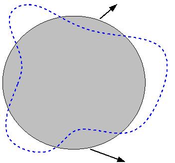
C
C
sr
X
X
tr
tr
w = sr
w
u
u
In the picture on the left v = w and on the right v = u.
C
C
sr
X
X
tr
tr
w = sr
w
u
u
Replacing s t by new demands s v and vt .
r r
r
r
Trivial to see E + R0 induces an Eulerian graph. Suppose G does not satisfy the cut condition
for the demand set R0. Let Y be a cut that violates the cut condition for R0. For this to happen
Y must be a tight set for R in G; this is the reason why replacing s t by s v and vt violates the
r r
r
r
cut condition for Y for R0. By complementing Y if necessary we can assume that v ∈ Y, s , t ∈/ Y .
r
r
Further, by Corollary 8, we can assume Y is central and hence Y ∩C is a contiguous segment of C.
By choice of r there is no demand r0 between Y − X and X − Y . If there was, then t would
r0
be closer to u than t . We have X, Y tight and
r
δR[X − Y, Y − X] = ∅.
We consider two cases. First, suppose X ∩ Y = ∅ (this is guaranteed if v = w). Then from
Corollary 10, X ∩ Y and X ∪ Y are tight since X ∩ Y = ∅ by assumption and X ∪ Y = V (since
t ∈ V \ (X ∪ Y )). X − Y = ∅, since s ∈ X − Y . Since X ∩ Y is a tight set and X ∩ Y = X, it
r
r
contradicts the choice of X as the tight set with X ∩ C minimal. If X ∩ Y = ∅ then v = u and
u ∈ Y ; again X ∪ Y = V . Note that the edge uw joins X and Y . In this case we claim that X ∪ Y
does not satisfy the cut condition which is a contradiction. To see this note that
|
δ (X ∪ Y )| ≤ |δ (X)| + |δ (Y )| − 2
G
G
G
since uw connects X to Y . However,
|
δ (X ∪ Y )| = |δ (X)| + |δ (Y )| = |δ (X)| + |δ (Y )|
H
H
H
G
G
C
C
sr
X
tr
tr
w = sr
w
u
u
Y
Y
Tight set Y in the two cases.
where the first inequality follows since X ∩ Y = ∅ and there are no demand edges between X − Y
and Y − X. The second inequality follows from the tightness of X and Y .
2
2
Sparse Cuts, Concurrent Multicomodity Flow and Flow-Cut
Gaps
In traditional combinatorial optimization, the focus has been on understanding and characterizing
those cases where cut condition implies existence of fractional/integral multiflow. However, as we
saw, even in very restrictive settings, cut condition is not sufficient. A theoretical CS/algorithms
perspective has been to quantify the “gap” between flow and cut. More precisely, suppose G
satisfies the cut condition for H. Is it true that there is a feasible multiflow in G that routes λdi
for each pair siti where λ is some constant in (0, 1)?
There are two reasons for considering the above. First, it is a mathematically interesting question.
Second, and this was the initial motivation from a computer science/algorithmic point of view, is to
obtain approximation algorithms for finding “sparse” cuts in graphs; these have many applications
in science and engineering. The following is known.
Theorem 12 Given a multiflow instance, it is co-NP complete to check if the cut-condition is
satisfied for the instance.
Definition 13 Given a multiflow instance the maximum concurrent flow for the given instance is
the maximum λ ≥ 0 such that there is a feasible multiflow if all demand values are multiplied by λ.
Proposition 14 There is a polynomial time algorithm that, given a multiflow instance, computes
the maximum concurrent flow.
Proof: Write a linear program:
max λ
flow for each siti ≥ λdi
Flow satisfies capacity constraints. We leave the details to the reader.
2
Definition 15 Given a multiflow instance on G, H, the sparsity of a cut U ⊂ V is
c (δ (U))
sparsity(U) :=
G
.
d (δH(U))
A sparsest cut is U ⊂ V such that sparsity(U) ≤ sparsity(U0) for all U0 ⊂ V . We refer to
min sparsity(U) as the min-sparsity of the given multiflow instance.
U⊂V
Observation 16 (G, H) satisfies the cut condition implies sparsity(U) ≥ 1 for all U ⊂ V .
Proposition 17 In many multiflow instance, if λ∗ is the max concurrent flow then
∗
( )
λ ≤ sparsity U , ∀U ⊂ V.
The ratio min−sparity is the flow cut gap for the given instance.
λ∗
For example,
with capacities and demands equal to 1, the flow-cut gap is 4. Min-sparsity for the above instance
3
is 1 while λ∗ = 3. In general, we are interested in quantifying flow-cut gaps for classes of instances
4
rather than a particular instance.
In the sequel, we think of G and H as ”topological” graphs in that they are not endowed with
capacities and demands. A multiflow instance on G, H is defined by c : E → R and d : R → R .
+
+
Note that by setting c(e) = 0 or d(r) = 0, we can “eliminate” some edges. We define α(G, H), the
flow-cut gap for G, H, as the supremum over all instances on G, H defined by capacities c : E → R
+
and d : R → R . We can then define for a graph G:
+
α(G) = sup (G, H).
H=(T,R)
T⊆V
Some results that we mentioned on the sufficiency of cut condition for feasible flow can be
restated as follows: α(G, H) = 1 if |R| = 2 (Hu’s theorem), α(G, H) = 1 if G is planar and T is the
vertex set of a face of G (Okamura-Seymour theorem), and so on. What can we say about α(G)
for an arbitrary graph?
Theorem 18 (Linial-London-Rabinovich, Aumann-Rabani) α(G) = O(log n) where n =
|
V | and in particular α(G, H) = O(log |R|) i.e. the flow-cut gap is O(log k) for k-commodity flow.
Moreover there exist graphs G, H for which α(G, H) = Ω(log |R|), in particular there exist graphs
G for which α(G) = Ω(log n).
Conjecture 19 α(G) = O(1) if G is a planar graph.
√
Theorem 20 (Rao) α(G) = O( log n) for a planar graph G.




References
[
1] Lex Schrijver, ”Combinatorial Optimization: Polyhedra and Efficiency”, Chapter 74, Vol. C,
Springer-Verlag, 2003.