实战PG vector 构建DBA 个人知识库之二: 向量数据库与 PG vector 介绍

开源软件联盟PostgreSQL分会 2024-09-03

500

作者

陈旭，捷银消费金融有限公司DBA

既第一篇实战PG vector构建DBA个人知识库之一：基础环境搭建以及大模型部署之后，

今天分享的是本系列之二：向量数据库与 PG vector 介绍

目前随着大模型的普及，向量数据库如雨后春笋版出现，首先是一些传统的NOSQL 像mongo, redis, es 发布版本支持，

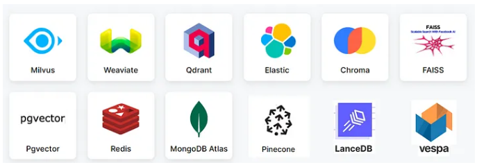
传统的老牌数据库干脆将23 C版本改名为 23 AI，MYSQL 甚至为了支持向量直接跳跃大版本发布了9.0. 市面上还有一些专门的向量数据库：FAISS、Milvus、Pinecone …

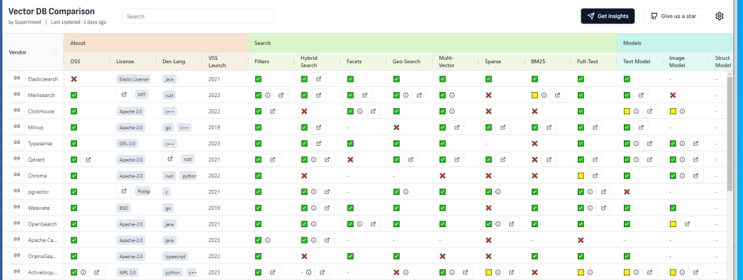
关于市面上向量数据库的比较可以参考: https://superlinked.com/vector-db-comparison

从这个榜单中，我们可以看到从不同的统计维度之间向量的数据库比较：

为什么要使用pg_vector做为我的向量数据库的方案呢？个人观点如下：
1.pg_vector 插件的方式支持向量，不需要单独安装一个全新的数据库，从而减少了机器，监控，运维，HA，灾备等等的一系列的成本。
2.不想NOSQL mongo. es 那样，你可以使用SQL的方式进行向量数据库操作
3.pg_vector 在国外已经大面积使用，深受广大程序员的喜爱，而且视频问文字资料相对较多。
4.基于传统老牌RDBMS, 保证数据库ACID特性
5.如果你的公司存在PG的数据库或者有PG经验DB的话，直接开箱即用

我们先安装一下PG数据库16.3版本，为了插件安装便利，我们选择源码安装, 下载地址： https://www.postgresql.org/ftp/source/v16.3/

[postgres@VM-24-9-centos postgres]$ wget https://ftp.postgresql.org/pub/source/v16.3/postgresql-16.3.tar.gz

编译安装软件

[root@VM-24-9-centos postgres]# su - postgres
Last login: Wed Jul 24 14:39:07 CST 2024 on pts/4
[postgres@VM-24-9-centos ~]$ tar -xvf postgresql-16.3.tar.gz
[postgres@VM-24-9-centos ~]$ cd /opt/postgres/
[postgres@VM-24-9-centos postgres]$ tar -xvf postgresql-16.3.tar.gz
[postgres@VM-24-9-centos postgresql-16.3]$ ./configure --prefix=/opt/pgsql-16  -with-ssl=openssl --with-pgport=5432
[postgres@VM-24-9-centos postgresql-16.3]$ make world -j16
[postgres@VM-24-9-centos postgresql-16.3]$ make install-world -j16

设置环境变量

PG_HOME='/opt/pgsql-16'
PATH=$PATH:$HOME/.local/bin:$HOME/bin:$PG_HOME/bin
alias psql='/opt/pgsql-16/bin/psql'
export PATH

初始化数据库

[postgres@VM-24-9-centos ~]$ /opt/pgsql-16/bin/initdb -A trust --data-checksums -D /data/pg5432/ -U postgres -W

启动数据库

[postgres@VM-24-9-centos ~]$  /opt/pgsql-16/bin/pg_ctl -D /data/pg5432/ -l logfile start
waiting for server to start.... done
server started
[postgres@VM-24-9-centos ~]$ psql
psql (16.3)
Type "help" for help.


postgres=#

为了日后的程序地址IP的连接畅通性，我们需要小改2个参数

postgres=# alter system set listen_addresses = '*';
ALTER SYSTEM
postgres=# select pg_reload_conf();
pg_reload_conf
----------------
t
(1 row)

HBA文件修改:
host    all             all             0.0.0.0/0              md5

以上我们完成了PG数据库的基本配置。

下面我们来看一下pgvector:
github上的下载地址： https://github.com/pgvector/pgvector

关于PG vector 的支持特性如下：

* exact and approximate nearest neighbor search
* single-precision, half-precision, binary, and sparse vectors
* L2 distance, inner product, cosine distance, L1 distance, Hamming distance, and Jaccard distance
* any language with a Postgres client

pgvector 下载

git clone --branch v0.7.3 https://github.com/pgvector/pgvector.git

pgvector的安装：

[postgres@VM-24-9-centos pgvector]$ make
[postgres@VM-24-9-centos pgvector]$ make install

创建vector 插件：我们可以看到关于插件的秒速支持向量类型，以及 ivfflat and hnsw 2种索引的搜索方式

postgres=# create extension vector;
CREATE EXTENSION
postgres=# \dx
                            List of installed extensions
 Name   | Version |   Schema   |                     Description                      
---------+---------+------------+------------------------------------------------------
plpgsql | 1.0     | pg_catalog | PL/pgSQL procedural language
vector  | 0.7.3   | public     | vector data type and ivfflat and hnsw access methods
(2 rows)

我们来创建一张含有vector类型的商品表：

CREATE TABLE product (
   id SERIAL PRIMARY KEY,
   name VECTOR(8)
);

手动插入一些数据：大致分为2大类：水果和球类

postgres=# insert into product(name,vec) values ('苹果','[0.11, 0.12, 0.13,0.14, 0.15, 0.16,0.17,0.18]');
INSERT 0 1
postgres=# insert into product(name,vec) values ('香蕉','[0.10, 0.13, 0.15,0.15, 0.16, 0.17,0.18,0.19]');
INSERT 0 1
postgres=# insert into product(name,vec) values ('足球','[3.31, 3.32, 3.33,3.34, 3.35, 3.36,3.37,3.18]');
INSERT 0 1
postgres=# insert into product(name,vec) values ('篮球','[3.10, 3.13, 3.15,3.15, 3.16, 3.17,3.18,3.19]');
INSERT 0 1

postgres=# select * from product;
id | name |                    vec
----+------+-------------------------------------------
 1 | 苹果 | [0.11,0.12,0.13,0.14,0.15,0.16,0.17,0.18]
 2 | 香蕉 | [0.1,0.13,0.15,0.15,0.16,0.17,0.18,0.19]
 3 | 足球 | [3.31,3.32,3.33,3.34,3.35,3.36,3.37,3.18]
 4 | 篮球 | [3.1,3.13,3.15,3.15,3.16,3.17,3.18,3.19]
(4 rows)

我们可以进行一个相似度的匹配: 我们采用大家初中数学学习的 cosine distance 计算距离。<=>：cosine distance

SELECT * FROM product
order by  vec <=> '[0.11, 0.12, 0.13,0.14, 0.15, 0.11,0.19,0.28]' limit 2;

pgvector 支持的一些向量距离的运算符：

<-> - L2 distance
<#> - (negative) inner product
<=> - cosine distance
<+> - L1 distance (added in 0.7.0)

到这里你可能会好奇怎样把具体的文字抽象成具体的向量数值呢？下面介绍一下 embedding 的概念。

An embedding is a numerical representation of a piece of information, for example, text, documents, images, audio, etc

我们可以看到针对人脸识别和视频鉴别的embedding 模型。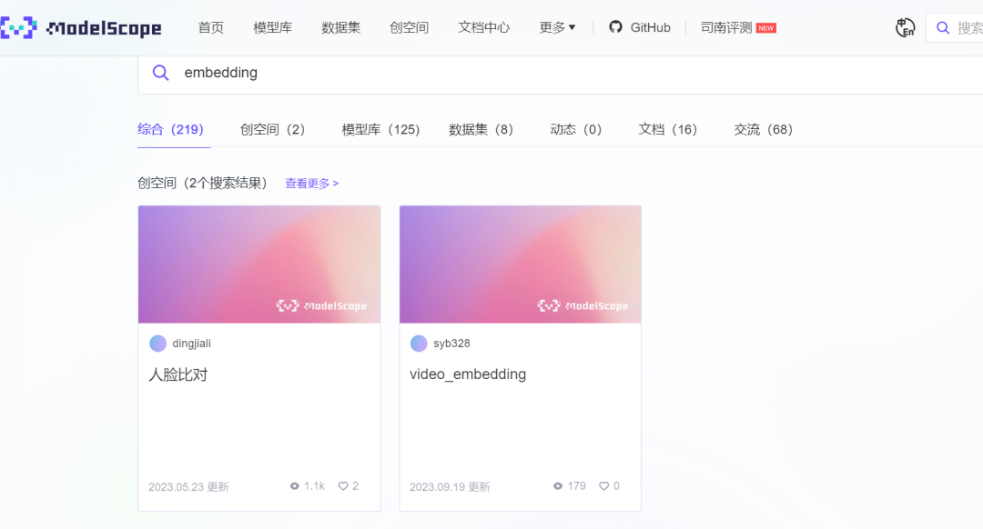

针对文本的向量生成embedding 模型有 text2vec-large-chinese： https://github.com/shibing624/text2vec?tab=readme-ov-file
简介: text2vec, text to vector. 文本向量表征工具，把文本转化为向量矩阵，实现了Word2Vec、RankBM25、Sentence-BERT、CoSENT等文本表征、文本相似度计算模型，开箱即用。

我们可以在python 环境中直接安装包

pip3 install SentenceModel
pip3 install psycopg3

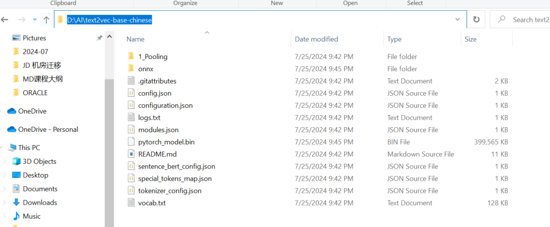
下载embedding model 模型文件：https://www.modelscope.cn/models/Jerry0/text2vec-base-chinese

我们下载到本地的电脑上：

Jason.ChenTJ@CN-L201098 MINGW64 /d/AI/MD课程大纲
$ git lfs install
Git LFS initialized.
Jason.ChenTJ@CN-L201098 MINGW64 /d/AI/MD课程大纲
$ git clone https://www.modelscope.cn/Jerry0/text2vec-base-chinese.git

测试文字生成向量数值：

from text2vec import SentenceModel
import  json
sentences = ['苹果']


model = SentenceModel("D:\\AI\\text2vec-base-chinese")
embeddings = model.encode(sentences)




print(json.dumps(embeddings.tolist()[0]))
print('dimension size of vector is: {}'.format(len(json.dumps(embeddings.tolist()[0]))))

默认生成的维度是 768个(In general, each sentence is translated to a 768-dimensional vector.)
输出：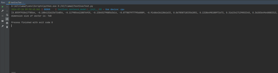

那我们现在试图写一个程序，把文本转换成向量写入到数据库pgvector中：

创建连接账户：

postgres=# create user app_vector password 'app_vector';
CREATE ROLE
postgres=# create schema app_vector authorization app_vector;
CREATE SCHEMA
postgres=# \c postgres app_vector
You are now connected to database "postgres" as user "app_vector".

创建表：

postgres=# \c postgres app_vector
You are now connected to database "postgres" as user "app_vector".
postgres=> create table product (id int , name text, embedding vector(768));
CREATE TABLE

写一段小程序load

from text2vec import SentenceModel
import psycopg2
import  json
def connect2PG():
   conn = psycopg2.connect(
       user="app_vector",
       password="app_vector",
       host="XX.XX.XXX.XX",
       port=5432,  # The port you exposed in docker-compose.yml
       database="postgres"
   )
   return conn
def execSQL(conn,sql):
   cur = conn.cursor()
   cur.execute(sql)
   conn.commit()
   cur.close()
   conn.close()
def generatedEmbedding(text):
   sentences = [text]
   model = SentenceModel("D:\\AI\\text2vec-base-chinese")
   embeddings = model.encode(sentences)
   return json.dumps(embeddings.tolist()[0])
   #print(json.dumps(embeddings.tolist()[0]))
   #print('dimension size of vector is: {}'.format(len(json.dumps(embeddings.tolist()[0]).split(","))))
def loadVec2DB(id,text):
   embeddings = generatedEmbedding(text)
   print(embeddings)
   sql =  """ insert into product(id,name,embedding) values({},'{}','{}')""".format(id,text,embeddings)
   print(sql)
   conn = connect2PG()
   execSQL(conn,sql)
if __name__ == '__main__':
    loadVec2DB(1,'苹果')
    loadVec2DB(2,'香蕉')

查看数据库：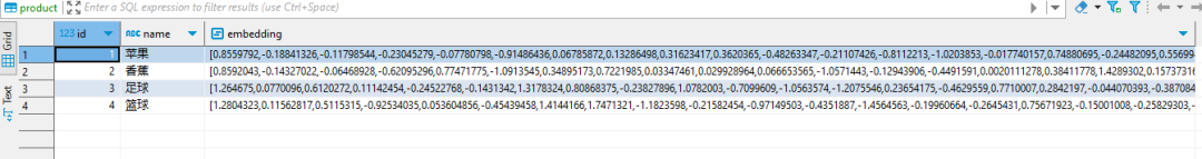

我们写一个相似度的查询SQL：

def querySimiliary(text):
   embeddings = generatedEmbedding(text)
   print(embeddings)
   sql = """
   SELECT id, name, 1 - (embedding <=> '{}') AS cosine_similarity
              FROM product
              ORDER BY cosine_similarity DESC LIMIT 2
   """.format(embeddings)
   conn = connect2PG()
   return querySQL(conn,sql)

我们查询一下：querySimiliary(“一种水果糖分高，黄色表皮”)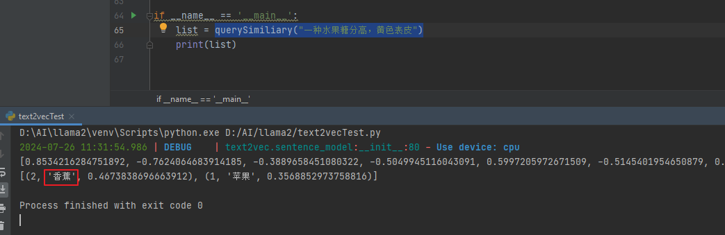

再次尝试：querySimiliary(“apple的中文是什么”)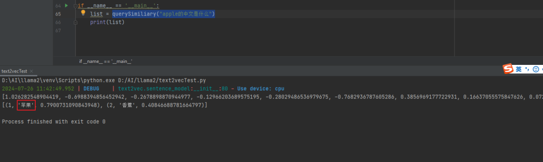

querySimiliary(“我要运动，有推荐的项目吗?”)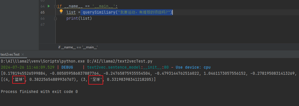

我们完成了python最数据库的基本操作后，下面我们看看vector 相关的索引：

hnsw类型索引：什么是HNSW呢？Hierarchical Navigable Small Word 网上基本上都翻译成：分层导航小世界

HNSW 是一种近似最近邻检索（ANN）索引。它基于图的性质旨在实现高效的搜索，尤其是在较大的数据规模下。HNSW 创建了一个多层次的图，每一层代表数据的一个子集，通过快速遍历这些层来找到近似最近邻。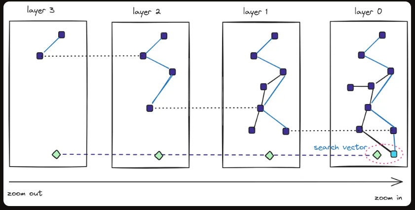

我们新建一张表，load进去一些数据，看一下执行查询语句的计划

postgres=> create table vector(id int, embeddings vector(3));
CREATE TABLE
postgres=> insert into vector  select generate_series(1,10),  STRING_TO_ARRAY(generate_series(1,10)||',1,2', ',')::int[];
INSERT 0 10
postgres=> select * from vector;
id | embeddings
----+------------
 1 | [1,1,2]
 2 | [2,1,2]
 3 | [3,1,2]
 4 | [4,1,2]
 5 | [5,1,2]
 6 | [6,1,2]
 7 | [7,1,2]
 8 | [8,1,2]
 9 | [9,1,2]
10 | [10,1,2]
(10 rows)

相似度查询：我们看到计划是Seq Scan on vector

postgres=> explain analyze SELECT * FROM vector ORDER BY embeddings <-> '[3,1,2]' LIMIT 1;
                                                   QUERY PLAN
------------------------------------------------------------------------------------------------------------------
Limit  (cost=32.23..32.23 rows=1 width=44) (actual time=0.026..0.026 rows=1 loops=1)
  ->  Sort  (cost=32.23..35.40 rows=1270 width=44) (actual time=0.025..0.025 rows=1 loops=1)
        Sort Key: ((embeddings <-> '[3,1,2]'::public.vector))
        Sort Method: top-N heapsort  Memory: 25kB
        ->  Seq Scan on vector  (cost=0.00..25.88 rows=1270 width=44) (actual time=0.011..0.014 rows=10 loops=1)
Planning Time: 0.055 ms
Execution Time: 0.044 ms
(7 rows)

我们在vector 这个列上创建一个hnsw类型的索引：

postgres=> CREATE INDEX ON vector USING hnsw (embeddings vector_l2_ops);
CREATE INDEX

再次查看执行计划：我们看到触发了之前我们创建的索引

postgres=> explain analyze SELECT * FROM vector ORDER BY embeddings <-> '[3,1,2]' LIMIT 1;
                                                             QUERY PLAN
---------------------------------------------------------------------------------------------------------------------------------------
Limit  (cost=8.07..8.49 rows=1 width=44) (actual time=0.031..0.032 rows=1 loops=1)
  ->  Index Scan using vector_embeddings_idx on vector  (cost=8.07..12.20 rows=10 width=44) (actual time=0.031..0.031 rows=1 loops=1)
        Order By: (embeddings <-> '[3,1,2]'::public.vector)
Planning Time: 0.088 ms
Execution Time: 0.053 ms
(5 rows)

对于hnsw 索引的创建有如下几种距离的计算方式：

L2 distance：CREATE INDEX ON items USING hnsw (embedding vector_l2_ops);
Inner product：CREATE INDEX ON items USING hnsw (embedding vector_ip_ops);
Cosine distance：CREATE INDEX ON items USING hnsw (embedding vector_cosine_ops);
L1 distance：CREATE INDEX ON items USING hnsw (embedding vector_l1_ops);
Hamming distance ：REATE INDEX ON items USING hnsw (embedding bit_hamming_ops);
Jaccard distance：CREATE INDEX ON items USING hnsw (embedding bit_jaccard_ops)

关于index 创建的参数选项：

m - the max number of connections per layer (16 by default)

m表示每一个图层layer中，点之间的相邻的最大个数，默认是16个，
增大M的值，意味着每个点有更多的邻居节点，从而加快了查询的速度，负面影响是创建的速度，磁盘和内存的开销

ef_construction - the size of the dynamic candidate list for constructing the graph (64 by default)

ef_construction 控制索引构建过程中使用的候选列表大小，默认是64个
理论上来说候选list 越大，index的质量越好，但是会增加索引构建的时间。

下面这幅图描述了hnsw 创建时间和参数ef_construction的关系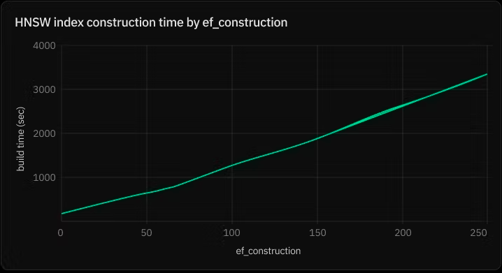

具体创建索引的语法参数是：

CREATE INDEX ON words USING hnsw (embedding vector_cosine_ops) WITH (m = 16, ef_construction = 64);

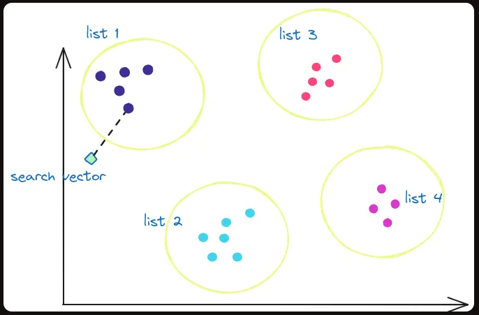
IVFFlat类型索引：Inverted File with Flat Indexing
IVFFlat结合了倒排文件和平坦索引的思想。它通过将数据集划分为多个list（或组），每个list维护一个倒排列表和一个平坦索引，用于快速搜索桶内的近邻。
It has faster build times and uses less memory than HNSW, but has lower query performance

我们创建一张表 vector2 并创建 IVFFlat类型索引:

postgres=>  create table vector2(id int, embedding vector(3));
CREATE TABLE
postgres=> insert into vector2  select generate_series(1,10000),  STRING_TO_ARRAY(generate_series(1,10000)||',1,2', ',')::int[];
INSERT 0 10000
postgres=> select count(1) from vector2;
count
-------
10000
(1 row)

创建IVFFlat类型索引：

postgres=> CREATE INDEX ON vector2 USING ivfflat (embedding vector_l2_ops) WITH (lists = 10);
CREATE INDEX

查看查询执行计划：

postgres=> explain analyze SELECT * FROM vector2 ORDER BY embedding <-> '[3,1,2]' LIMIT 1;
                                                                 QUERY PLAN
----------------------------------------------------------------------------------------------------------------------------------------------
Limit  (cost=22.50..22.53 rows=1 width=29) (actual time=0.404..0.406 rows=1 loops=1)
  ->  Index Scan using vector2_embedding_idx2 on vector2  (cost=22.50..313.50 rows=10000 width=29) (actual time=0.402..0.404 rows=1 loops=1)
        Order By: (embedding <-> '[3,1,2]'::vector)
Planning Time: 2.915 ms
Execution Time: 0.447 ms
(5 rows)

关于IVFFlat 索引创建的2个参数说明：

list : Choose an appropriate number of lists - a good place to start is rows 1000 for up to 1M rows and sqrt(rows) for over 1M rows
list 是创建索引的时候指定的参数从数值通常选取表大小/1000 (1百万业内)，（大于1百万的话）采用sqrt(rows)

probes: When querying, specify an appropriate number of probes (higher is better for recall, lower is better for speed) - a good place to start is sqrt(lists)
probes：索引查询的时候设置的参数（数值小速度快，数值大recall好），最佳起始值为sqrt(rows)

postgres=> set ivfflat.probes =100;
SET
postgres=> explain analyze SELECT * FROM vector2 ORDER BY embedding <-> '[3,1,2]' LIMIT 1;
                                                                 QUERY PLAN
-----------------------------------------------------------------------------------------------------------------------------------------------
Limit  (cost=205.00..205.04 rows=1 width=29) (actual time=9.330..9.334 rows=1 loops=1)
  ->  Index Scan using vector2_embedding_idx2 on vector2  (cost=205.00..586.00 rows=10000 width=29) (actual time=9.328..9.332 rows=1 loops=1)
        Order By: (embedding <-> '[3,1,2]'::vector)
Planning Time: 0.146 ms
Execution Time: 9.546 ms
(5 rows)

这个参数默ivfflat.probes 认是1

postgres=> reset ivfflat.probes;
RESET
postgres=> show ivfflat.probes;
ivfflat.probes
----------------
1
(1 row)


postgres=> explain analyze SELECT * FROM vector2 ORDER BY embedding <-> '[3,1,2]' LIMIT 1;
                                                                 QUERY PLAN
----------------------------------------------------------------------------------------------------------------------------------------------
Limit  (cost=22.50..22.53 rows=1 width=29) (actual time=0.412..0.413 rows=1 loops=1)
  ->  Index Scan using vector2_embedding_idx2 on vector2  (cost=22.50..313.50 rows=10000 width=29) (actual time=0.411..0.411 rows=1 loops=1)
        Order By: (embedding <-> '[3,1,2]'::vector)
Planning Time: 0.095 ms
Execution Time: 0.438 ms
(5 rows)

可以看出ivfflat.probes = 1 数值越小，执行查询的时间越快。Execution Time: 0.438 ms(ivfflat.probes = 1) vs Execution Time: 9.546 ms (ivfflat.probes =100)

最后我们横向的比较一下2种索引的构建时间和查询效率的比较：

数据量基数为1000万：max_parallel_maintenance_workers TO 4 和 set maintenance_work_mem=’8GB’ 条件下

hnsw: index 创建时间05:41.715 (4个并行和8GB的内存)

postgres=> create table vector_hnsw(id int, embedding vector(3));
CREATE TABLE
Time: 19.506 ms
postgres=> insert into vector_hnsw  select generate_series(1,10000000),  STRING_TO_ARRAY(generate_series(1,10000000)||',1,2', ',')::int[];
INSERT 0 10000000
Time: 22864.818 ms (00:22.865)
postgres=> SET max_parallel_maintenance_workers TO 4;
SET
Time: 0.269 ms
postgres=> set maintenance_work_mem='8GB';
SET
Time: 0.198 ms
postgres=> CREATE INDEX ON vector_hnsw USING hnsw (embedding vector_l2_ops);
CREATE INDEX
Time: 341715.259 ms (05:41.715)

表大小和hnsw 索引的大小：可以索引大小是表的6倍左右。3037 MB/498 M = 6

表大小：
postgres=> select pg_size_pretty(pg_relation_size('vector_hnsw'));
pg_size_pretty
----------------
498 MB
(1 row)

索引大小：
postgres=> select pg_size_pretty(pg_total_relation_size('vector_hnsw')-pg_relation_size('vector_hnsw'));
pg_size_pretty
----------------
3037 MB
(1 row)


Time: 0.909 ms
postgres=> select 3037/498;
?column?
----------
        6
(1 row)

我们再来看一下 ivfflat: index 创建时间 04:34.026 (4个并行和8GB的内存)

postgres=> create table vector_ivfflat(id int, embedding vector(3));
CREATE TABLE
Time: 8.332 ms
postgres=> insert into vector_ivfflat  select generate_series(1,10000000),  STRING_TO_ARRAY(generate_series(1,10000000)||',1,2', ',')::int[];
INSERT 0 10000000
Time: 21212.166 ms (00:21.212)
postgres=> SET max_parallel_maintenance_workers TO 4;
SET
Time: 0.296 ms
postgres=> set maintenance_work_mem='8GB';
SET
Time: 0.211 ms
postgres=> select sqrt(10000000);
        sqrt
--------------------
3162.2776601683795
(1 row)


Time: 1.175 ms
postgres=> CREATE INDEX ON vector_ivfflat USING ivfflat (embedding vector_l2_ops) WITH (lists = 3200);


CREATE INDEX
Time: 274025.837 ms (04:34.026)

表大小和ivfflat 索引的大小：索引（357 MB）比表（498 MB）略小

postgres=> select pg_size_pretty(pg_relation_size('vector_ivfflat'));
pg_size_pretty
----------------
498 MB
(1 row)


Time: 1.527 ms
postgres=> select pg_size_pretty(pg_total_relation_size('vector_ivfflat')-pg_relation_size('vector_ivfflat'));
pg_size_pretty
----------------
357 MB
(1 row)


Time: 0.989 ms

最后看一下单条SQL的查询效率：果然在查询性能上会精掉你的下巴：
Index Scan using vector_ivfflat_embedding_idx：Execution Time: 2879.538 ms
Index Scan using vector_hnsw_embedding_idx：Execution Time: 6.373 ms

至少在我的实验环境中 hnsw 类型的索引性能要远远好于vfflat 类型的索引

postgres=> explain analyze SELECT * FROM vector_ivfflat ORDER BY embedding <-> '[3,1,2]' LIMIT 1;
                                                                              QUERY PLAN

---------------------------------------------------------------------------------------------------
-------------------------------------------------------------------
Limit  (cost=45.94..45.94 rows=1 width=29) (actual time=2841.296..2841.300 rows=1 loops=1)
   ->  Index Scan using vector_ivfflat_embedding_idx on vector_ivfflat  (cost=45.94..31179.19 rows=
10000000 width=29) (actual time=2841.292..2841.293 rows=1 loops=1)
         Order By: (embedding <-> '[3,1,2]'::vector)
Planning Time: 0.097 ms
Execution Time: 2879.538 ms
(5 rows)

postgres=> explain analyze SELECT * FROM vector_hnsw ORDER BY embedding <-> '[3,1,2]' LIMIT 1;
                                                                        QUERY PLAN

---------------------------------------------------------------------------------------------------
--------------------------------------------------------
Limit  (cost=10.84..10.87 rows=1 width=29) (actual time=6.233..6.246 rows=1 loops=1)
   ->  Index Scan using vector_hnsw_embedding_idx on vector_hnsw  (cost=10.84..252400.84 rows=10000
000 width=29) (actual time=6.230..6.231 rows=1 loops=1)
         Order By: (embedding <-> '[3,1,2]'::vector)
Planning Time: 0.628 ms
Execution Time: 6.373 ms
(5 rows)

至此我们总结一下2种类型索引的对比：

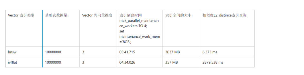
从上述对比的表格中，我们可以看出:
1.索引创建时间上，HNSW的构建时间要略长于ivfflat
2索引空间比上，由于hnsw是基于graph 多个layer 构建的，索引需要更大的空间，设置是表大小很多倍
3.单条查询效率上hnsw 远远好于ivfflat , hnsw 甚至适合于OLAP类型的查询，ivflat 适合OLAP类型的查询报表。
4.此外相对于传统btree索引，向量索引在构建过程中对数据库内存，CPU资源要求更高。在索引创建过程中如果内存资源不足会产生提示：

postgres=> CREATE INDEX ON vector_hnsw USING hnsw (embedding vector_l2_ops);
NOTICE:  hnsw graph no longer fits into maintenance_work_mem after 6146391 tuples
DETAIL:  Building will take significantly more time.
HINT:  Increase maintenance_work_mem to speed up builds.

最后我们总结一下：
1.市面上的向量数据库种类繁多, 可以参考一下向量数据库之间的比较，以及表达了DBA选择向量数据库的观点：按照实际的项目需求选择你熟悉的数据库
2.pgvector 的安装以及使用以及整合embedding model 进行向量数据的插入和相似度查询
3.关于vector 2种索引类型 hnsw 和 ivfflat 测试和比较：优先选择 hnsw 更适合业务系统，相对于传统的btree索引，需要考虑到硬件资源加大投入的问题尤其是内存和磁盘空间。

Have a fun 🙂 !

文章转载自开源软件联盟PostgreSQL分会，如果涉嫌侵权，请发送邮件至：contact@modb.pro进行举报，并提供相关证据，一经查实，墨天轮将立刻删除相关内容。

实战PG vector 构建DBA 个人知识库之二: 向量数据库与 PG vector 介绍

评论