PolarDB 基于代价的查询改写技术解析（三）

ZzzMickey 2024-10-22

266

对CBO的调用

前面已提到，在MySQL的常规优化流程中，完成查询改写操作后会进入CBO的模块（对应JOIN::optimize函数），执行每个query block的物理优化，这个过程中，基于统计信息+代价模型，MySQL会基于代价，考虑每个query block内部可能的单表访问方式、join顺序、join算法等，从中选择代价最低的最优方案。这种计算代价的能力，对于CBQT也是非常重要的，因为我们需要有“基于代价决定改写是否应用”的能力，也就是说在枚举过程中，如果一个改写不确定是否会更优，需要能够让CBO告知改写前/后的代价，通过比较来决定。这就要求我们能够在迭代过程中反复调用CBO组件，理论上把它当做一个黑盒，一个可以计算代价的黑盒。

CBO的抽象与精简

MySQL的原始CBO组件是非常重的，熟悉MySQL代码的同学应该了解JOIN::optimize函数中完成的工作，除了计算代价，他还需要做一系列事前、事后的动作，包括：

等值、常量传递和一些类型转换处理等
计算必要统计信息
枚举最优计划并计算代价
生成物理执行计划

整个过程很长，如果我们把这些都包含进来，势必造成枚举过程效率过低，因此第一个动作就是对CBO做抽象和精简，实现一个Mini-CBO的组件，它只做为计算代价的最小化动作，尽可能降低调用的开销。我们把Mini-CBO实现为一个黑盒，传递给它一个query plan的子树，返回这颗子树的最优代价。

CBO的重入与复用

对于Mini-CBO的反复调用，也暴露了一些进一步提升效率的机会，即从各个粒度上，实现对代价计算的复用，尽量避免执行重复的优化过程。这个粒度从小到大是：

Table level，对于每个table，MySQL会基于谓词，考虑可能的range访问方式，这个过程中会估算range scan要扫描的行数，而这是通过index dive的动态采样来完成的，我们通过缓存+复用dive的结果，即可以节省反复读取page的开销，也可以避免由于采样导致的优化效果不稳定问题。
Join level，对于一个连续的join序列+join条件，也会缓存其对应的最佳join方式和join代价，后续再遇到直接获取对应代价值，避免了昂贵的join顺序枚举。
Query Block level，当一个输入的query tree子树中，一些query block与之前计算过的block相同，我们也会复用之前计算的结果，更大幅度提升重入的效率。
Query Tree Level，query block level的复用一定程度上也意味着query tree的局部复用

Query Tree的复制

在前面介绍枚举框架的图中，我们看到一个object，会同时考虑应用一个改写rule或不应用该rule，这是基于query tree的clone能力来实现的。具体来说，当Rewriter考虑对一个object应用当前改写Rule时，会先对整个query tree做一次clone，生成一个新tree，并基于新tree完成改写动作，然后将新tree输入到Mini-CBO中计算代价，同时原有的不做改写的tree也会进入Mini-CBO计算代价，通过比较两个结果，保留2颗query tree的一个作为winner，进入下一个步骤。

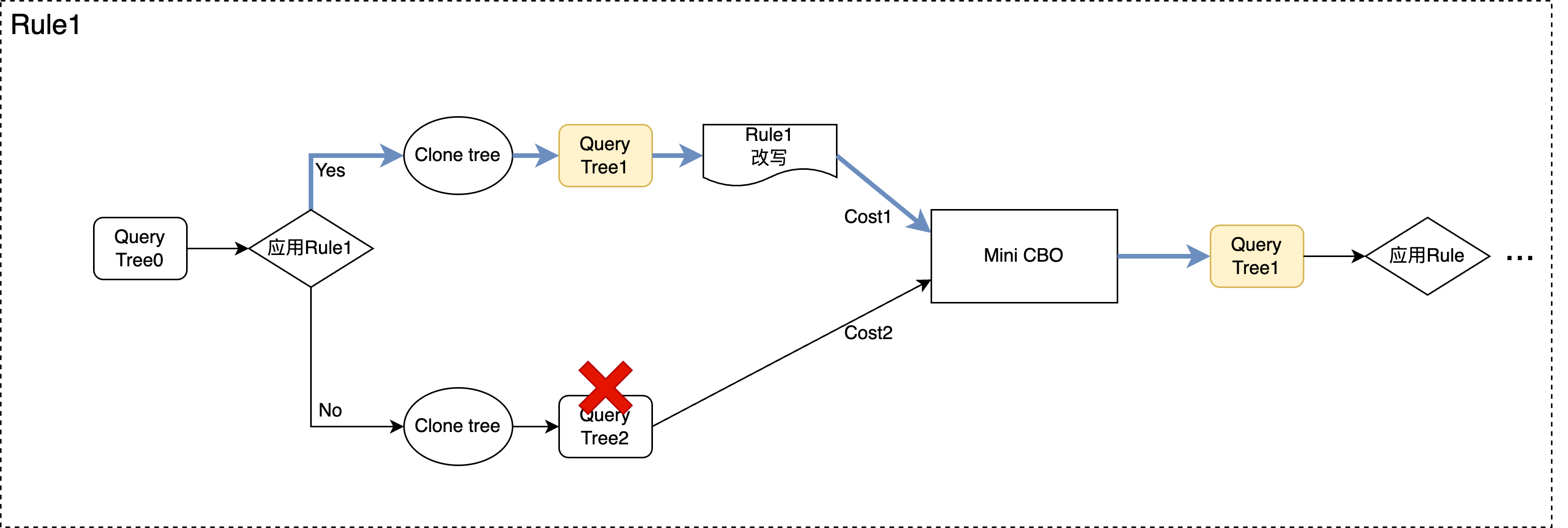
从query tree的角度来看，流程如上图，对于每个需要基于代价确定的改写规则，都需要经过Mini-CBO的”裁决”来选中winner。当然从原理和工程上，这里还有很多要处理的事情，例如

基于启发式的改写规则与基于代价的改写规则如何交互和影响
基于代价的规则之间的Interleaving和Juxtaposition （可参考Oracle paper）
流程中针对clone的优化

这些细节这里就不赘述了。

示例

目前我们实现了标量子查询转物化表、GroupBy解关联子查询、物化表合并、子查询折叠等四种基于代价的变换规则以及子查询转SemiJoin、window_function解关联子查询等八种启发式变换规则。下面使用TPCH的数据构造两个场景说明CBQT框架的优势。测试环境为PolarDB线上实例，规格为polar.mysql.g2.large（4C8G)；测试数据为TPCH 1G的数据。

自动选择代价更低的计划

以TPCH Q17为例。 Q17查询为：

select
  sum(l_extendedprice) / 7.0 as avg_yearly
from
  lineitem,
  part
where
  p_partkey = l_partkey
  and p_brand = 'Brand#12'
  and p_container = 'JUMBO BOX'
  and l_quantity < (
    select
      0.2 * avg(l_quantity)
    from
      lineitem
    where
      l_partkey = p_partkey
  )
limit 1;

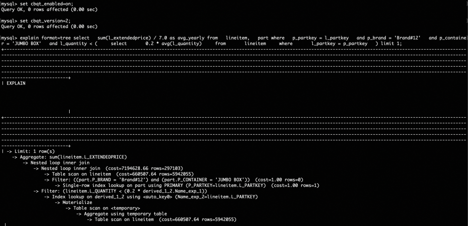
对于这个查询，子查询可以直接按照语义以关联的形式迭代执行或者通过GroupBy解关联后进行执行，而何种方式性能更好取决于具体场景，比如索引、数据量等。在TPCH-1G数据下，没有二级索引时，Q17通过GroupBy解关联执行的效率是更高的，对比如下。 关联执行 计划：

mysql> explain format=tree select   sum(l_extendedprice) / 7.0 as avg_yearly from   lineitem,   part where   p_partkey = l_partkey   and p_brand = 'Brand#12'   and p_container = 'JUMBO BOX'   and l_quantity < (     select       0.2 * avg(l_quantity)     from       lineitem     where       l_partkey = p_partkey   ) limit 1;
+-----------------------------------------------------------------------------------------------------------------------------------------------------+
| EXPLAIN                                                                                                                                           
+-----------------------------------------------------------------------------------------------------------------------------------------------------+
| -> Limit: 1 row(s)
    -> Aggregate: sum(lineitem.L_EXTENDEDPRICE)
        -> Nested loop inner join  (cost=7194628.66 rows=297103)
            -> Table scan on lineitem  (cost=660507.64 rows=5942055)
            -> Filter: ((part.P_BRAND = 'Brand#12') and (part.P_CONTAINER = 'JUMBO BOX') and (lineitem.L_QUANTITY < (select #2)))  (cost=1.00 rows=0)
                -> Single-row index lookup on part using PRIMARY (P_PARTKEY=lineitem.L_PARTKEY)  (cost=1.00 rows=1)
                -> Select #2 (subquery in condition; dependent)
                    -> Aggregate: avg(lineitem.L_QUANTITY)
                        -> Filter: (lineitem.L_PARTKEY = part.P_PARTKEY)  (cost=125722.69 rows=594206)
                            -> Table scan on lineitem  (cost=125722.69 rows=5942055)

执行时间：7579.54s

解关联执行 计划：

mysql> explain format=tree select   sum(l_extendedprice) / 7.0 as avg_yearly from   lineitem,   part where   p_partkey = l_partkey   and p_brand = 'Brand#12'   and p_container = 'JUMBO BOX'   and l_quantity < (     select       0.2 * avg(l_quantity)     from       lineitem     where       l_partkey = p_partkey   ) limit 1;
+-----------------------------------------------------------------------------------------------------------------------+
| EXPLAIN                                                                                                               
+-----------------------------------------------------------------------------------------------------------------------+
| -> Limit: 1 row(s)
    -> Aggregate: sum(lineitem.L_EXTENDEDPRICE)
        -> Nested loop inner join
            -> Nested loop inner join  (cost=7194628.66 rows=297103)
                -> Table scan on lineitem  (cost=660507.64 rows=5942055)
                -> Filter: ((part.P_BRAND = 'Brand#12') and (part.P_CONTAINER = 'JUMBO BOX'))  (cost=1.00 rows=0)
                    -> Single-row index lookup on part using PRIMARY (P_PARTKEY=lineitem.L_PARTKEY)  (cost=1.00 rows=1)
            -> Filter: (lineitem.L_QUANTITY < (0.2 * derived_1_2.Name_exp_1))
                -> Index lookup on derived_1_2 using <auto_key0> (Name_exp_2=lineitem.L_PARTKEY)
                    -> Materialize
                        -> Table scan on <temporary>
                            -> Aggregate using temporary table
                                -> Table scan on lineitem  (cost=660507.64 rows=5942055)

执行时间：25.45s

可以看到解关联执行只需要25s左右，性能是不解关联执行的数百倍。如果在各个表上有二级索引，那么不解关联的性能会更好，对比如下。

解关联执行 计划：

mysql> explain format=tree select   sum(l_extendedprice) / 7.0 as avg_yearly from   lineitem,   part where   p_partkey = l_partkey   and p_brand = 'Brand#12'   and p_container = 'JUMBO BOX'   and l_quantity < (     select       0.2 * avg(l_quantity)     from       lineitem     where       l_partkey = p_partkey   ) limit 1;
+-------------------------------------------------------------------------------------------------------------------------+
| EXPLAIN                                                                                                                 
+-------------------------------------------------------------------------------------------------------------------------+
| -> Limit: 1 row(s)
    -> Aggregate: sum(lineitem.L_EXTENDEDPRICE)
        -> Nested loop inner join
            -> Nested loop inner join  (cost=40024.75 rows=57147)
                -> Filter: ((part.P_BRAND = 'Brand#12') and (part.P_CONTAINER = 'JUMBO BOX'))  (cost=19835.90 rows=1930)
                    -> Table scan on part  (cost=19835.90 rows=192989)
                -> Index lookup on lineitem using LINEITEM_FK2 (L_PARTKEY=part.P_PARTKEY)  (cost=7.50 rows=30)
            -> Filter: (lineitem.L_QUANTITY < (0.2 * derived_1_2.Name_exp_1))
                -> Index lookup on derived_1_2 using <auto_key0> (Name_exp_2=part.P_PARTKEY)
                    -> Materialize
                        -> Group aggregate: avg(lineitem.L_QUANTITY)
                            -> Index scan on lineitem using LINEITEM_FK2  (cost=593311.60 rows=5799036)

执行时间：20.58s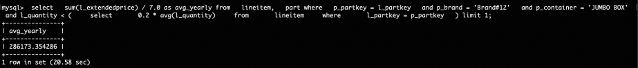

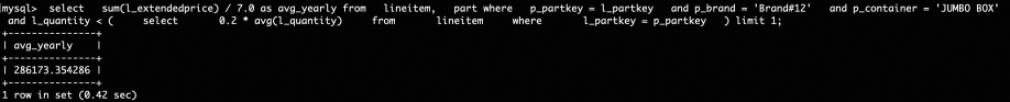
关联执行 计划：

mysql> explain format=tree select   sum(l_extendedprice) / 7.0 as avg_yearly from   lineitem,   part where   p_partkey = l_partkey   and p_brand = 'Brand#12'   and p_container = 'JUMBO BOX'   and l_quantity < (     select       0.2 * avg(l_quantity)     from       lineitem     where       l_partkey = p_partkey   ) limit 1;
+---------------------------------------------------------------------------------------------------------------------+
| EXPLAIN                                                                                                             
+---------------------------------------------------------------------------------------------------------------------+
| -> Limit: 1 row(s)
    -> Aggregate: sum(lineitem.L_EXTENDEDPRICE)
        -> Nested loop inner join  (cost=40024.75 rows=57147)
            -> Filter: ((part.P_BRAND = 'Brand#12') and (part.P_CONTAINER = 'JUMBO BOX'))  (cost=19835.90 rows=1930)
                -> Table scan on part  (cost=19835.90 rows=192989)
            -> Filter: (lineitem.L_QUANTITY < (select #2))  (cost=7.50 rows=30)
                -> Index lookup on lineitem using LINEITEM_FK2 (L_PARTKEY=part.P_PARTKEY)  (cost=7.50 rows=30)
                -> Select #2 (subquery in condition; dependent)
                    -> Aggregate: avg(lineitem.L_QUANTITY)
                        -> Index lookup on lineitem using LINEITEM_FK2 (L_PARTKEY=part.P_PARTKEY)  (cost=10.46 rows=30)

执行时间：0.42s
  
可以看到解关联执行的查询性能相对关联执行的查询性能下降明显。

而CBQT框架能够根据查询代价自动确定是否采用解关联执行，对于上述场景下的Q17。 在有索引时的计划选择为：
  
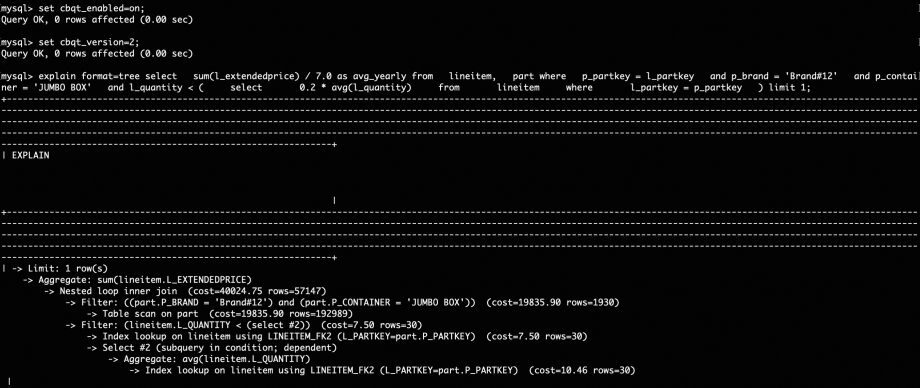
在没有索引时的选择为：
  
可以看到CBQT都能够自动选出最优的计划，不需要DBA基于经验人工对不同场景单独进行配置。

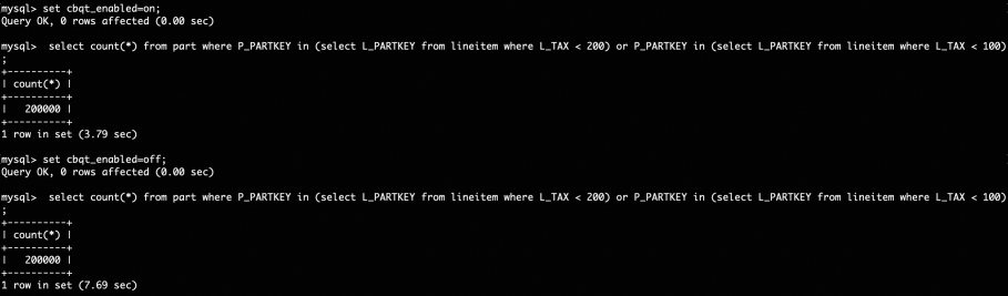
反复枚举变换
CBQT框架的另一个优势在于能够变换规则是反复枚举的，某些不可用的变换规则在其他规则应用后可能变得可用了，从而可以选出一个更优的计划，
例如下述查询：

SELECT *
FROM part
WHERE P_PARTKEY IN (
		SELECT L_PARTKEY
		FROM lineitem
		WHERE L_TAX < 100
	)
	OR P_PARTKEY IN (
		SELECT L_PARTKEY
		FROM lineitem
		WHERE L_TAX < 200
	);
由于两个子查询是由OR连接的，因此在PolarDB中无法直接转为semijoin，如果不做任何变换其计划如下：

mysql> explain format=tree select count(*) from part where P_PARTKEY in (select L_PARTKEY from lineitem where L_TAX < 100) or P_PARTKEY in (select L_PARTKEY from lineitem where L_TAX < 200);
+----------------------------------------------------------------------------------------------------------------------------------------------------------------------------------------------+
| EXPLAIN                                                                                                                                                                                      
+----------------------------------------------------------------------------------------------------------------------------------------------------------------------------------------------+
| -> Aggregate: count(0)
    -> Filter: (<in_optimizer>(part.P_PARTKEY,part.P_PARTKEY in (select #2)) or <in_optimizer>(part.P_PARTKEY,part.P_PARTKEY in (select #3)))  (cost=20310.00 rows=198050)
        -> Index scan on part using PRIMARY  (cost=20310.00 rows=198050)
        -> Select #2 (subquery in condition; run only once)
            -> Filter: ((part.P_PARTKEY = `<materialized_subquery>`.L_PARTKEY))
                -> Limit: 1 row(s)
                    -> Index lookup on <materialized_subquery> using <auto_distinct_key> (L_PARTKEY=part.P_PARTKEY)
                        -> Materialize with deduplication
                            -> Filter: (lineitem.L_TAX < 100.00)  (cost=555350.80 rows=1808695)
                                -> Table scan on lineitem  (cost=555350.80 rows=5426628)
        -> Select #3 (subquery in condition; run only once)
            -> Filter: ((part.P_PARTKEY = `<materialized_subquery>`.L_PARTKEY))
                -> Limit: 1 row(s)
                    -> Index lookup on <materialized_subquery> using <auto_distinct_key> (L_PARTKEY=part.P_PARTKEY)
                        -> Materialize with deduplication
                            -> Filter: (lineitem.L_TAX < 200.00)  (cost=555350.80 rows=1808695)
                                -> Table scan on lineitem  (cost=555350.80 rows=5426628)
但是可以观察到这两个子查询只有WHERE条件不一样，因此可以做子查询的折叠，折叠后的查询形式如下：
SELECT *
FROM part
WHERE P_PARTKEY IN (
		SELECT L_PARTKEY
		FROM lineitem
		WHERE L_TAX < 100 OR L_TAX < 200
	);
子查询折叠后的计划如下：
mysql> explain format=tree  select count(*) from part where P_PARTKEY in (select L_PARTKEY from lineitem where L_TAX < 100) or P_PARTKEY in (select L_PARTKEY from lineitem where L_TAX < 200);
+----------------------------------------------------------------------------------------------------------------------------------------------------------------------------------------------+
| EXPLAIN                                                                                                                                                                                     
+----------------------------------------------------------------------------------------------------------------------------------------------------------------------------------------------+
| -> Aggregate: count(0)
    -> Filter: <in_optimizer>(part.P_PARTKEY,part.P_PARTKEY in (select #3))  (cost=20310.00 rows=198050)
        -> Index scan on part using PRIMARY  (cost=20310.00 rows=198050)
        -> Select #3 (subquery in condition; run only once)
            -> Filter: ((part.P_PARTKEY = `<materialized_subquery>`.L_PARTKEY))
                -> Limit: 1 row(s)
                    -> Index lookup on <materialized_subquery> using <auto_distinct_key> (L_PARTKEY=part.P_PARTKEY)
                        -> Materialize with deduplication
                            -> Filter: ((lineitem.L_TAX < 100.00) or (lineitem.L_TAX < 200.00))  (cost=555350.80 rows=3014552)
                                -> Table scan on lineitem  (cost=555350.80 rows=5426628)
此时只有一个子查询了，符合了子查询转semijoin的条件，因此可以进一步变换为semijoin的形式，其计划如下：
mysql> explain format=tree  select count(*) from part where P_PARTKEY in (select L_PARTKEY from lineitem where L_TAX < 100) or P_PARTKEY in (select L_PARTKEY from lineitem where L_TAX < 200);
+--------------------------------------------------------------------------------------------------------------------------------------------------------------------------------------------+
| EXPLAIN                                                                                                                                                                                   
+--------------------------------------------------------------------------------------------------------------------------------------------------------------------------------------------+
| -> Aggregate: count(0)
    -> Nested loop inner join
        -> Filter: (part.P_PARTKEY is not null)  (cost=20310.00 rows=198050)
            -> Index scan on part using PRIMARY  (cost=20310.00 rows=198050)
        -> Single-row index lookup on <subquery3> using <auto_distinct_key> (L_PARTKEY=part.P_PARTKEY)
            -> Materialize with deduplication
                -> Filter: ((lineitem.L_TAX < 100.00) or (lineitem.L_TAX < 200.00))  (cost=555350.80 rows=3014552)
                    -> Table scan on lineitem  (cost=555350.80 rows=5426628)
在TPCH-1G数据量下，对于该查询，使用CBQT框架进行改写的效果对比如下图：

可以看到使用CBQT框架进行改写后，查询性能提升了接近一倍。
展望
新的改写框架目前在PolarDB 8.0.22版本已上线，可以通过cbqt_enabled开关做总体的开启和关闭，此外类似optimizer_switch，我们也提供了cbqt_rule_switch这个参数，来控制各个改写动作是否在CBQT框架中生效。 目前的改写框架已基本成型，但还有很多事情需要做，这个框架是PolarDB新一代查询优化器的基础设施，其后续能支持的功能是非常灵活宽广的。一些近期/中期的目标如下：
持续增加更多的查询改写能力，覆盖更多用户场景，提升查询执行效果
优化Rewriter枚举过程中的效率，通过引入Partial Clone等能力降低复制和CBO的代价
利用反复枚举的能力，实现针对PolarDB异构引擎异构计划在优化过程中的融合，更高效的生成针对多引擎的混合执行计划，例如找到最优的行/列存混合计划形态
…

polardb

文章转载自ZzzMickey，如果涉嫌侵权，请发送邮件至：contact@modb.pro进行举报，并提供相关证据，一经查实，墨天轮将立刻删除相关内容。