


点击上方【蓝色】字体 关注我们


01 场景描述
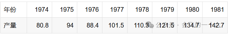
(1)试用趋势移动平均法来建立布的年产量预测模型。
建立布的直线指数平滑预测模型。
(3)计算模型拟合误差,比较三个模型的优劣。
02
符号规定与基本假设
符号规定
假设布的产量不受机器生产技术影响;
03 模型的分析与建立
(1) 建立布的年产量预测模型
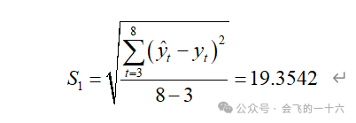
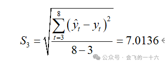
(2) 预测的标准误差为
(3) 二次指数平滑法的计算公式为
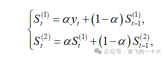
(4) 其中, 表示一次指数的平滑值;
 表示二次指数的平滑值

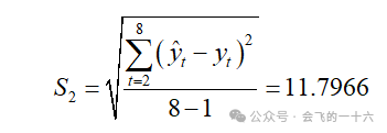
若  则预测的标准误差为
04 模型求解【基于SQL实现】
4.1 数据准备
create table production as(select stack(8,'1974', '80.8','1975', '94.0','1976', '88.4','1977', '101.5','1978', '110.3','1979', '121.5','1980', '134.7','1981', '142.7') as (years, production));
4.2 问题分析
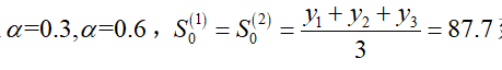
步骤1:计算初始值
select years, production, casewhen rn = 1 then cast(avg(production)over (order by years rows between current row and 2 following ) as decimal(18, 4)) end init_production, rnfrom (select years, production, row_number() over (order by years) rnfrom production) t
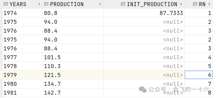
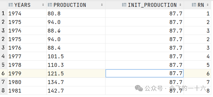
对计算得到的初始值进行NULL值补全,便于后续计算。得到如下SQL
select years, production, last_value(init_production ignore nulls) over (order by YEARS) init_production, rnfrom (select years, production, casewhen rn = 1 then cast(avg(production)over (order by years rows between current row and 2 following ) as decimal(18, 1)) end init_production, rnfrom (select years, production, row_number() over (order by years) rnfrom production) t) t
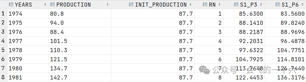
步骤2:计算一次平滑值
平滑值计算公式如下:


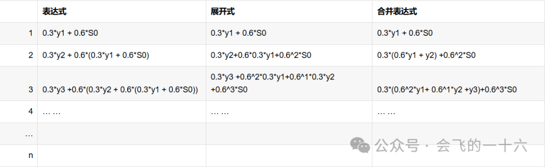
经过上述演绎,我们总结通项公式如下:

对上述迭代公式分析,我们可以看出指数平滑方法会将更大的权重赋到最近的观测值,对于更久远的观测值则会赋予较小的权重,权重的衰减速度由参  数控制。这里权重
  会以指数方式逐渐衰减到0。 对于0到1之间的任何 值,随着时间向前推移,观察值的权重呈指数型下降,因此我们称之为“指数平滑”。当越大时权重衰减的越快。当越小时权重衰减的越慢,当
 ,
,  的极端情况,指数平滑的预测值等于最后一个预测值。
通过通项公式,我们就很容易利用SQL语言去求解,从而避免了复杂的递归运算。要解决上述公式中第一项,且能够控制项数(n -i)我们自然相到用自关联形式得到全量数据集后再进行行行比较。其中的求解我们用power(x,n)函数,结果值保留四位小数,分别计算当  及 时的一次平滑值。具体SQL如下:
with init as (select years, production, last_value(init_production ignore nulls) over (order by YEARS) init_production, rnfrom (select years, production, casewhen rn = 1 then cast(avg(production)over (order by years rows between current row and 2 following ) as decimal(18, 1)) end init_production, rnfrom (select years, production, row_number() over (order by years) rnfrom production) t) t)--计算一次平滑值, s1 as (select t1.years, t1.production, t1.init_production, t1.rn, cast(sum(case when t2.rn <= t1.rn then t2.production * power(0.7, t1.rn - t2.rn) else 0 end) * 0.3 +power(0.7, t1.rn) * t1.init_production as decimal(18, 4)) s1_p3, cast(sum(case when t2.rn <= t1.rn then t2.production * power(0.4, t1.rn - t2.rn) else 0 end) * 0.6 +power(0.4, t1.rn) * t1.init_production as decimal(18, 4)) s1_p6from init t1,init t2group by t1.years, t1.production, t1.init_production, t1.rn)select *from s1order by YEARS;
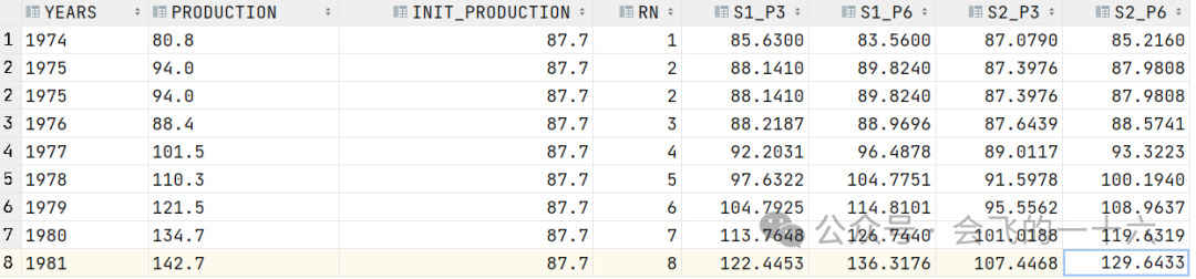
步骤3:计算二次平滑值
with init as (select years, production, last_value(init_production ignore nulls) over (order by YEARS) init_production, rnfrom (select years, production, casewhen rn = 1 then cast(avg(production)over (order by years rows between current row and 2 following ) as decimal(18, 1)) end init_production, rnfrom (select years, production, row_number() over (order by years) rnfrom production) t) t)--计算一次平滑值, s1 as (select t1.years, t1.production, t1.init_production, t1.rn, cast(sum(case when t2.rn <= t1.rn then t2.production * power(0.7, t1.rn - t2.rn) else 0 end) * 0.3 +power(0.7, t1.rn) * t1.init_production as decimal(18, 4)) s1_p3, cast(sum(case when t2.rn <= t1.rn then t2.production * power(0.4, t1.rn - t2.rn) else 0 end) * 0.6 +power(0.4, t1.rn) * t1.init_production as decimal(18, 4)) s1_p6from init t1,init t2group by t1.years, t1.production, t1.init_production, t1.rn)--计算二次平滑值, s2 as (select t1.years, t1.production, t1.init_production, t1.rn, t1.s1_p3, t1.s1_p6, cast(sum(case when t2.rn <= t1.rn then t2.s1_p3 * power(0.7, t1.rn - t2.rn) else 0 end) * 0.3 +power(0.7, t1.rn) * t1.init_production as decimal(18, 4)) s2_p3, cast(sum(case when t2.rn <= t1.rn then t2.s1_p6 * power(0.4, t1.rn - t2.rn) else 0 end) * 0.6 +power(0.4, t1.rn) * t1.init_production as decimal(18, 4)) s2_p6from s1 t1,s1 t2group by t1.years, t1.production, t1.init_production, t1.rn, t1.s1_p3, t1.s1_p6)select *from s2order by YEARS;
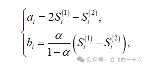
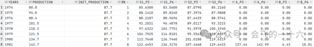
步骤4:计算直线趋势模型的系数 及
及
with init as (select years, production, last_value(init_production ignore nulls) over (order by YEARS) init_production, rnfrom (select years, production, casewhen rn = 1 then cast(avg(production)over (order by years rows between current row and 2 following ) as decimal(18, 1)) end init_production, rnfrom (select years, production, row_number() over (order by years) rnfrom production) t) t)--计算一次平滑值, s1 as (select t1.years, t1.production, t1.init_production, t1.rn, cast(sum(case when t2.rn <= t1.rn then t2.production * power(0.7, t1.rn - t2.rn) else 0 end) * 0.3 +power(0.7, t1.rn) * t1.init_production as decimal(18, 4)) s1_p3, cast(sum(case when t2.rn <= t1.rn then t2.production * power(0.4, t1.rn - t2.rn) else 0 end) * 0.6 +power(0.4, t1.rn) * t1.init_production as decimal(18, 4)) s1_p6from init t1,init t2group by t1.years, t1.production, t1.init_production, t1.rn)--计算二次平滑值, s2 as (select t1.years, t1.production, t1.init_production, t1.rn, t1.s1_p3, t1.s1_p6, cast(sum(case when t2.rn <= t1.rn then t2.s1_p3 * power(0.7, t1.rn - t2.rn) else 0 end) * 0.3 +power(0.7, t1.rn) * t1.init_production as decimal(18, 4)) s2_p3, cast(sum(case when t2.rn <= t1.rn then t2.s1_p6 * power(0.4, t1.rn - t2.rn) else 0 end) * 0.6 +power(0.4, t1.rn) * t1.init_production as decimal(18, 4)) s2_p6from s1 t1,s1 t2group by t1.years, t1.production, t1.init_production, t1.rn, t1.s1_p3, t1.s1_p6)--计算直线趋势模型系数select years, production, init_production, rn, s1_p3, s1_p6, s2_p3, s2_p6, cast(case when rk=1 then 2*s1_p3 - s2_p3 else 0 end as decimal(18,2)) a_p3, cast(case when rk=1 then 2*s1_p6 - s2_p6 else 0 end as decimal(18,2)) a_p6, cast(case when rk=1 then (s1_p3 - s2_p3)*(0.3/(1-0.3)) else 0 end as decimal(18,2)) b_p3, cast(case when rk=1 then (s1_p6 - s2_p6)*(0.6/(1-0.6)) else 0 end as decimal(18,2)) b_p6from (select years, production, init_production, rn, s1_p3, s1_p6, s2_p3, s2_p6, row_number() over (order by rn desc) rkfrom s2) t;
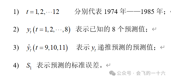
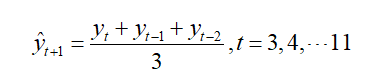
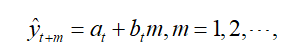
步骤5:构建线性预测模型进行结果预测


4.3 结果分析及问题讨论
本题第一问建立出布的年产量预测模型为。本体第二问建立布的直线指数预测模型为。本题第三问从标准差的角度考虑,选择 的二次指数平滑模型。本题第四问选用 的二次指数平滑模型作为最优化的模型得到1982年和1985年的产量预测值为153 亿米和183.03亿米 。
(1)本模型适合场景:产量预测、计划需求预测、企业营收预测等
(2)对于平滑系数的确定
在指数平滑法中,预测成功的关键是a的选择。a的大小规定了在新预测值中新数据和原预测值所占的比例。a值愈大,新数据所占的比重就愈大,原预测值所占比重就愈小,反之亦然。
对于平滑系数的选取,阅读相关文献后,你会发现一些经验值:
(1)当需求历史比较稳定时,选择较小的α值,0.05~0.2;
当需求历史有波动,但长期趋势没有大的变化时,可选择稍大的α值,0.1~0.4;
(2)当需求历史波动很大,呈现明显且迅速的上升或下降趋势时,宜选取较大的α值,0.6~0.8;
(3)当需求历史是上升或者下降序列时,α宜取较大值,0.6~1。
(4)但是,需求多稳定才算稳定,波动多大才算大,这很难量化,各人理解也不相同。比如有家企业的营收每年翻倍,计划经理认为业务波动很大,在她的逻辑里,增长本身就意味着波动,α应该取0.6~0.8。但我研究了一些产品后,发现α实际上取0.3最合适,也就是说业务的变动没有想象的大。
在具体实践中,平滑系数可按以下方式择优:
(1)先把需求历史做成折线图,时间为横轴,需求历史为纵轴,大致判断需求历史的稳定性,以及是否有趋势、季节性;(2)然后参照上述经验值,确定平滑系数的大致范围;(3)最后套用几个不同的α值,一般每个相差0.05,看哪个的预测准确度最高,哪个就是最优的平滑系数。这一般会通过复盘的方式进行,比如复盘过去13周的预测,计算每周的均方误差,然后求得13周的平均均方误差,据此判断预测的准确度。(3) 的选择
的选择
对于我们可以有两种选择方法:
选取第一个时刻的实际值作为。
使用前N个实际值的平均值作为。
(4) 指数平滑法的缺点:
(1)对数据的转折点缺乏鉴别能力,但这一点可通过调查预测法或专家预测法加以弥补。(2)长期预测的效果较差,故多用于短期预测。
(5) 指数平滑法的优点:
1)对不同时间的数据的非等权处理较符合实际情况。2)实用中仅需选择一个模型参数a 即可进行预测,简便易行。3)具有适应性,也就是说预测模型能自动识别数据模式的变化而加以调整。
05 小 结
文章通过纺织生产布料的年产量预测这一场景进行引入,利用二次指数平滑法构建线性预测模型 该模型的实现主要采用SQL语言,通过均方根误差(RMSE)分析表明,当平滑系数时,模型误差较小,相对准确。
在备品备件领域,特别是高值慢动的产品,需求很不频繁,一旦发生,往往意味着很多(小概率事件不容易发生,一旦发生则意味着不再是小概率事件):是不是这批设备用到一定年限了,需要更换相应的备件,或者产线在做什么预防性维修等。简单指数平滑法能够更迅速地捡起这一信号,尽快调整预测,驱动供应链尽快响应。
指数平滑法未来挑战
(1)简单指数平滑法虽然只有一个系数,但该平滑系数的优化不易。常见的误区是高估业务的变动性,取较大的平滑系数,灵敏度是足够了,但有可能过度反应,放大“杂音”,降低预测准确度。
(2)简单指数平滑法适合短期预测,比如适合预测下一期的补货。但如果预测的时段长了,虽然我们假定未来每期的需求都一样,都等于下一期的预测,但时间跨度越长,这个假定越难成立。
(3)跟移动平均法一样,简单指数平滑法是滞后的,一旦需求表现出趋势、季节性等,指数平滑法就一直处于“追赶”状态,我们得考虑更合适的指数平滑模型,比如霍尔特指数平滑(趋势)模型和霍尔特–温特(季节性加趋势)模型。
附录:预测通项公式完整推导过程
最简单的指数平滑方法被称为“简单指数平滑”,这种方法适用于预测没有明显趋势或季节特征的数据。简单指数平滑通过一个递归式来获取所有观测数据的权重,并在此基础上做出对未来的预测。简单指数平滑的递归式定义:

如果我们将上面的递归式展开可以得到如下的等式:
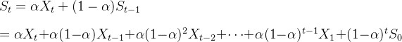

预测公式:

 :表示t+h 时刻的预测值即
 : 表示时刻 t 的实际观测值.
 是平滑参数
是平滑参数 
 : 它是递归展开式的初始化参数。
如果您觉得本文还不错,对你有帮助,那么不妨可以关注一下我的数字化建设实践之路专栏,这里的内容会更精彩。
专栏 原价99,现在活动价59.9,按照阶梯式增长,还差5个人上升到69.9,最终恢复到原价。


会飞的一十六
扫描右侧二维码关注我们
点个【在看】 你最好看

