Window function 的实现(2)

SQL SERVER 中 window function 的实现

由于上述约束，SQL SERVER 对 window function 的支持程度没有 mysql 高；但是因为有了“窗口的起始和结束位置都与 current row 的数据没有关系”这个约束， SQL SERVER 对 window function 的实现非常简洁，对 IMCI的实现有一定的参考意义，因此这里做一个简单描述。

不带 frame 的 window function

在没有指定 frame 的时候（e.g., SUM(profit) OVER(PARTITION BY country))，window expression 的作用范围是整个 partition，因此 window function 的实现相对简单，只要将输入数据分区，然后计算 window expression 即可；例如下面的 SQL：

SELECT
year,
country,
product,
profit,
SUM(profit) OVER(PARTITION BY country) AS country_profit
FROM
sales;

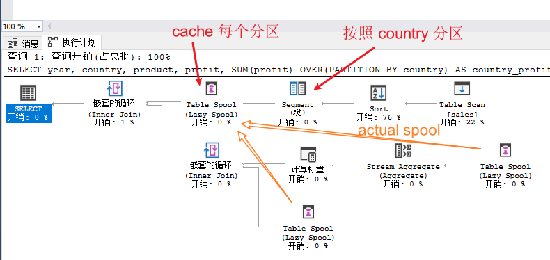
在 SQL SERVER 里面，执行计划如下：

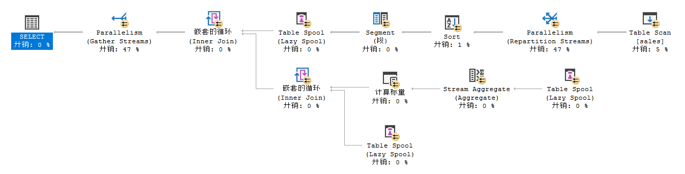
并行的执行计划加了 exchange:

其中比较关键的两个算子是 Segment 和 Table Spool：

1. Segment 用于对输入数据进行分区，分成不同的“segment”；在上面的 query 里面，会按照 window 里面的 country 这一列进行分区；这个 Segment 类似于 IMCI 的 HashJoin 和 HashGroupby 里面的 partition，区别在于这个 Segment 算子依赖于前面的 Sort 算子做“streaming”的分区，而 IMCI 的 partition 直接用 hash 的方式进行分区，速度上会有一些优势；
2. Table Spool 用于“cache”输入的数据，类似于 IMCI 的 Materialize 算子，区别在于：
   1. table spool 有 lazy spool 和 eager spool 的区别，lazy spool 只会被动 cache 那些“流经它的数据”；
   2. spool 下面如果是 segement 算子，则会有“segment spool”的行为，下面会描述；
   3. spool 算子有 primary spool 和非 primary spool 的区分；primary spool 是真正保存数据的，非 primary spool 则是对 primary spool 的引用；上图中，上面的 spool 是 primary spool，下面两个 spool 是非 primary spool；区分这两种 spool 的一个用处是，可以保持一个树状的执行计划，而不是有 common child 的 DAG；比如一个 query 如果在多个地方引用了同一个 VIEW，那么只需要一个地方物化这个 VIEW（i.e., primary spool），其他地方引用这个 spool 就行（非 primary spool）；又比如在子查询的处理中，也可以这么处理 shared sub-plan；

这个执行计划的执行过程是：

1. table scan -> sort -> segment 首先将数据分区
2. table spool 的每次 fetch from segment，都会取一个完整的 segment
3. 顶层的 nested loop join 驱动下面 nested loop join 执行

下面的 nested loop join 的 predicate 是 true，其子节点分别

• 1. 从 table spool 中取每个 segment （i.e., 每个 partition）的数据，进行 stream aggregate（i.e., SUM(profit)）；
  2. 从 table spool 中取每个 segment

将两个子节点 join 起来，就可以得到一个 partition 的结果集；

需要说明的是：

1. 真正对每个 partition 进行运算的是第二个 nested loop join，第一个 nested loop join （i.e., SELECT 后面那个）只是为了驱动 table scan -> sort -> segment -> table spool 这条 pipeline，将每个 segment 保存到 spool 里面；
2. 这里的 table spool 下面挂着一个 segment 算子，因此每次 cache 都只是 cache 一个“分区”

带 frame 的 window function

在指定 frame 的 window function 里面，当窗口移动到下一行，窗口的范围都会随之改变，因此如何在这种情况下快速计算不同窗口的值，就需要一定技巧。

与 MySQL 不同的是，在 SQL SERVER 的 window function 里面，“窗口的起始和结束位置都与 current row 的数据没有关系”，也就是说，

1. 窗口是定长的，或者
2. 窗口从 partition 的第一行/最后一行开始不断扩张/缩小（e.g, ROWS BETWEEN UNBOUNDED PRECEDING AND CURRENT ROW)

因此在带 frame 的 window function 里面，SQL SERVER 使用一个 “window spool”来实现。例如下面的 SQL：

SELECT
year,
country,
product,
profit,
SUM(profit) OVER(
PARTITION BY country
ORDER BY profit
ROWS BETWEEN 3 PRECEDING and CURRENT ROW --- 窗口范围是前三行到当前行
) AS country_profit0
FROM
sales;

在这个例子里面，窗口的访问是前三行到当前行，其执行计划是：

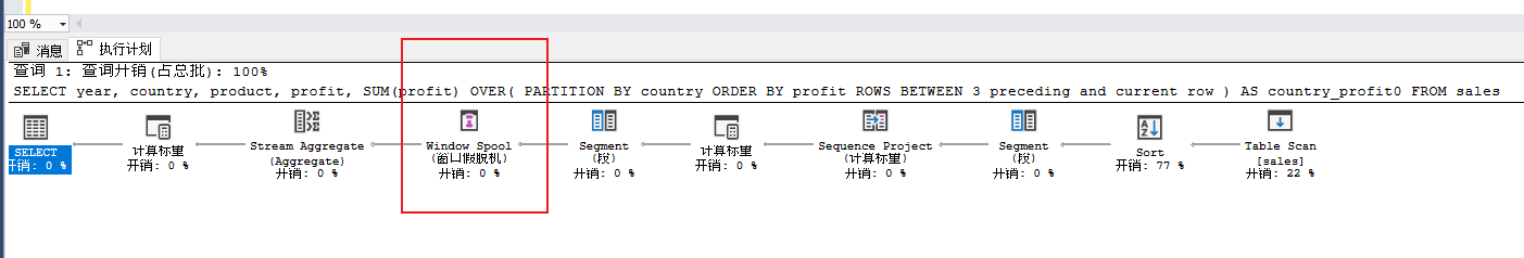
其中的 window spool 的主要作用是：

1. 将 segment 中的每个分区 cache 住（与上文的 table spool 类似）；
2. 在往上吐数据时，为每个 window 的数据增加一个 “WindowCount”，使得同一个 window 中的行拥有相同的 WindowCount，可以被聚合到一起；

例如，对于如下属于同一个分区的数据：

+------+---------+---------+--------+
| year | country | product | profit |
+------+---------+---------+--------+
| 1999 | FINLAND | P0 | 100 |
| 2000 | FINLAND | P1 | 100 |
| 2001 | FINLAND | P2 | 100 |
| 2002 | FINLAND | P3 | 100 |
| 2003 | FINLAND | P4 | 100 |
| 2004 | FINLAND | P5 | 100 |
+------+---------+---------+--------+

Window spool 向上吐数据时，其中一个方式是：

第 1 次吐数据：
+------+---------+---------+--------+-------------+
| year | country | product | profit | WindowCount |
+------+---------+---------+--------+-------------+
| 1999 | FINLAND | P0 | 100 | 1 |
+------+---------+---------+--------+-------------+

第 2 次吐数据：
+------+---------+---------+--------+-------------+
| year | country | product | profit | WindowCount |
+------+---------+---------+--------+-------------+
| 1999 | FINLAND | P0 | 100 | 2 |
| 2000 | FINLAND | P1 | 100 | 2 |
+------+---------+---------+--------+-------------+

第 3 次吐数据：
+------+---------+---------+--------+-------------+
| year | country | product | profit | WindowCount |
+------+---------+---------+--------+-------------+
| 1999 | FINLAND | P0 | 100 | 3 |
| 2000 | FINLAND | P1 | 100 | 3 |
| 2001 | FINLAND | P2 | 100 | 3 |
+------+---------+---------+--------+-------------+

第 4 次吐数据：
+------+---------+---------+--------+-------------+
| year | country | product | profit | WindowCount |
+------+---------+---------+--------+-------------+
| 1999 | FINLAND | P0 | 100 | 4 |
| 2000 | FINLAND | P1 | 100 | 4 |
| 2001 | FINLAND | P2 | 100 | 4 |
| 2002 | FINLAND | P3 | 100 | 4 |
+------+---------+---------+--------+-------------+

第 5 次吐数据：
+------+---------+---------+--------+-------------+
| year | country | product | profit | WindowCount |
+------+---------+---------+--------+-------------+
| 2000 | FINLAND | P1 | 100 | 5 |
| 2001 | FINLAND | P2 | 100 | 5 |
| 2002 | FINLAND | P3 | 100 | 5 |
| 2003 | FINLAND | P4 | 100 | 5 |
+------+---------+---------+--------+-------------+

（当然，也可以把这个 5 次合并成一次）

由于每个 window 的 WindowCount 是相同的，因此上面的 stream aggr 只需要 group by WindowCount 就可以得到正确的结果。

不难看出，因为做了重复运算，因此这里的复杂度是 O(N * M)，N 是数据量，M 是窗口长度。

对多个 window function 的处理

当一个 query block 里面出现多个 window function 时，e.g.,：

SELECT
col0,
col1,
window_expr0(...) over (window0),
window_expr1(...) over (window1)
FROM
tables;

SQL SERVER 的处理方法是：

1. 当多个 window function 里面的 window 定义相同时，做合并（e.g., 使用同一个 window spool）；
2. 当多个window function 里面的 window 定义不同时（e.g., partition columns 不同，或者 frame 的定义不同），在一个 window spool 上叠加另一个 window spool。

其他数据库中 window function 的实现

window function 三要素（partition、order、frame）中 partition 、sort 的处理都比较通用（要么是排序要么是哈希，同时考虑上并行处理时的如何对数据分区），因此这里忽略。

不同数据库对 frame 的处理却不太一样，这里简单描述一下：

POSTGRESQL

在窗口移动的过程中保存一个 “running aggregation”，因此对于那种不断扩张的窗口定义（e.g., range between unbounded preceding and current row），有加速作用；但是对于定长的移动窗口（e.g., sum(b) over (order by a rows between 5 preceding and 5 following)），作用不大；

(注：从 paper 里面读的，没有读代码）

MYSQL

从 mysql80 的 sql/sql_executor.cc 文件的里 process_buffered_windowing_record() 这个函数上方的长注释大概可以看出 mysql 的处理和优化逻辑：

1. 对于 range between unbounded preceding and current row 这种可以用 running aggregation 的情况，使用 running aggregation；
2. 对于 sum(b) over (order by a rows between 5 preceding and 5 following) 这种定长窗口移动，且 window expression 是 SUM / AVG 等函数时，可以在窗口移动的时候，把上一个窗口的边界值去掉（i.e, Removable Cumulative Aggregation）；这种优化在某些情况下会有精度问题，因此可以通过 windowing_use_high_precision 这个开关选择是否打开；
3. 对于其他的情况，利用一个 window buffer，在窗口移动的时候将数据拷到这个 buffer 里面，然后算 window expression；这种算法 worst case 的复杂度还是 O(n * m), n 是数据量，m 是窗口的最大长度；

看起来 mysql 的优化还是比较到位的。

ORACLE

暂时没找到相关资料。

HYPER

对于常见窗口定义，维持“running aggregation”，或者 “Removable Cumulative Aggregation”，来快速得到window expression 的值；对于其他情况，利用一个线段树（segment tree）来保证无论窗口如何变化，使得取某一个窗口的 window expression 值，最多只需 log n 的时间，因此 worst case 的性能是 O(n log(n))； 参考 《Efficient Processing of Window Functions in Analytical SQL Queries》这篇 paper。

这种方式既不会影响一般情况下的性能，又能够限制 worst case 的复杂度，是比较好的处理方式。