【Python的机器学习】预测未来股价（二）

数据信息化 2019-11-24

941

机器学习之路

预测未来股价（二）

首先我们要对得到的股票行情信息进行数据清洗，将数据中的空值写成-99999，并定义预测的天数。这样将数据喂给机器时，机器会比对其他正常的数据，判别出此为异常值。代码如下：

future_value='close'
df.fillna(value=-99999,inplace=True)    #填充数据中空值为-99999，检测时剔除异常值
far_forecast=int(math.ceil(0.01*len(df)))  #预测的天数变成整数
print(far_forecast)

打印结果，可以看到预测天数正好为7，也就是一周：

接下来对收盘价做偏移，作为未来七天的预测值的标签：

df['label']=df[future_value].shift(-far_forecast) #将7天的收盘价格放到预测的label上
df.dropna(inplace=True) #删除掉shift偏移为空的值
#print(df)
print(df.head(10))
print(df.tail())

可以看到收盘价已做偏移，并且最后含有Null值的数据也被删掉了：

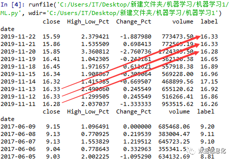
接下来我们要定义变量以及贴上对应的标签。从上面的数据可以看到每行的数据相差较大，从-1.887980到773473.50，所以我们要做数据标准化处理：

x = np.array(df.drop(['label'],1)) #只保留close，High_Low_Pct，Change_Pct，volume等变量
x = preprocessing.scale(x)    # 将数据集标准化处理，使预处理量纲保持一致
x_Recent_Real_Data = x[-far_forecast:] #只用尾部的部分来做预测


y = np.array(df['label'])

进行交叉验证，用75%的数据进行训练：

x_train,x_test,y_train,y_test = train_test_split(x,y,test_size=0.25) #进行交叉验证，设置测试数据预留25%，不断洗牌，避免结果有偏见

下面将采用两种算法，来看下机器预测的准确度：

算法一（线性回归算法：LinearRegression）：

具体算法数学模型请看：

https://blog.csdn.net/lilong_csdn/article/details/81937496

代码如下：

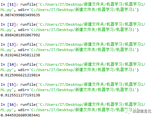
black_box = LinearRegression() #采用线性回归算法
black_box.fit(x_train,y_train) #适配过程转化，将训练数据喂给机器
forecast_set=black_box.predict(x_Recent_Real_Data)    #用尾部数据做测试
#print(forecast_set)
#print(df.tail(7))
accuracy = black_box.score(x_test,y_test)   #对比模拟数据，显示正确率
print(accuracy)

可以看到预测的正确率高达94%：

算法二（支持向量机算法：Support Vector Machine）：

具体算法数学模型请看：

https://blog.csdn.net/u011630575/article/details/78916747

代码如下：

black_box = svm.SVR()#采用支持向量机算法
black_box.fit(x_train,y_train) #适配过程 转化


forecast_set=black_box.predict(x_Recent_Real_Data)
#print(forecast_set)
#print(df.tail(7))


accuracy = black_box.score(x_test,y_test)   #对比模拟数据，显示正确率
print(accuracy)

这里注意在调用svm算法的时候，可能以为版本的原因出现warning，要去除显示添加代码：

import warnings
 
warnings.filterwarnings("ignore", category=FutureWarning, module="sklearn", lineno=193) #忽略警告

可以看到预测的正确率高达87%：

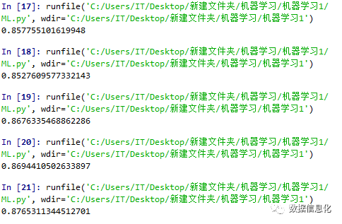
虽然这两种算法的准确率都达到了80%以上，但是实际情况按照预测的股价来买的话肯定是赔钱的，这是因为机器预测只是一个大致的方向，而实际收盘价会在此方向上下浮动。

代码全量展示：

import pandas as pd
import tushare as ts
import math
import numpy as np
from sklearn import preprocessing, svm
from sklearn.model_selection import train_test_split
from sklearn.linear_model import LinearRegression


import warnings
 
warnings.filterwarnings("ignore", category=FutureWarning, module="sklearn", lineno=193) #忽略警告


df=ts.get_hist_data('000001')
df=df[['open','high','close','low','volume']]


df['High_Low_Pct']=(df['high']-df['low'])/df['low']*100  #增幅比：（最高价-最低价）/最低价
df['Change_Pct']=(df['close']-df['open'])/df['open']*100 #涨幅比：(收盘价-开盘价）/开盘价


df=df[['close','High_Low_Pct','Change_Pct','volume']]


pd.set_option('display.max_rows',1000)
pd.set_option('display.max_columns',1000)


#print(df.head(20))


future_value='close'
df.fillna(value=-99999,inplace=True)    #填充数据中空值为-99999，检测时剔除异常值
far_forecast=int(math.ceil(0.01*len(df)))  #预测的天数变成整数
#print(far_forecast)


df['label']=df[future_value].shift(-far_forecast) #将7天的收盘价格放到预测的label上
df.dropna(inplace=True) #删除掉shift偏移为空的值
#print(df)
#print(df.head(10))
#print(df.tail())


x = np.array(df.drop(['label'],1)) #只保留close，High_Low_Pct，Change_Pct，volume等变量
x = preprocessing.scale(x)    # 将数据集标准化处理，使预处理量纲保持一致


x_Recent_Real_Data = x[-far_forecast:] #只用尾部的部分来做预测
y = np.array(df['label'])


x_train,x_test,y_train,y_test = train_test_split(x,y,test_size=0.25) #进行交叉验证，设置测试数据预留25%，不断洗牌，避免结果有偏见


#black_box = LinearRegression() #采用线性回归算法
black_box = svm.SVR()#采用支持向量机算法
black_box.fit(x_train,y_train) #适配过程 转化


forecast_set=black_box.predict(x_Recent_Real_Data)
#print(forecast_set)
#print(df.tail(7))


accuracy = black_box.score(x_test,y_test)   #对比模拟数据，显示正确率
print(accuracy)

下一章我们将继续深度研究支持向量机算法（Support Vector Machine），并且窥探黑盒（black_box）中到底发生了什么，通过可视化形象来展现。

下一章：【Python的机器学习】支持向量机算法（三）

python 机器学习

文章转载自数据信息化，如果涉嫌侵权，请发送邮件至：contact@modb.pro进行举报，并提供相关证据，一经查实，墨天轮将立刻删除相关内容。

【Python的机器学习】预测未来股价（二）

评论