机器学习 | 《统计学习方法》001. 感知机实现

数苗铺子 2021-07-06

678

前言

今天来跟大家一起学一下李航老师《统计学习方法》这本书中感知机模型，本系列推文不会设计太多的理论知识（理论部分请看原书），旨在学习如何使用python实现书中的模型。

1. 感知机基本内容

1.1 感知机简介

感知机是一种二分类模型，其输入为实例的特征，输出为实力的类别，旨在求出将训练数据进行线性划分的分离超平面。其最早在1957年由Rosenblant提出，是神经网络与支持向量机的基础。

1.2 感知机的定义

定义 2.1（感知机）：假设输入空间（特征空间）为，输出空间为。输入表示实例的特征向量，对应于输入空间(特征空间)的点；输出表示实例的类别。由输入空间到输出空间的如下函数：

称为感知机。其中w和b为感知机模型参数，叫做权值(weight)或权值向量(weight vector)，叫作偏置(bias)，表示w和x的内积。sign是符号函数，即：

1.3 感知机学习的策略：

假设训练数据集是线性可分的，感知机学习的目标是求得一个能够将训练集正实例点和复实例点完全正确分开的分离超平面。其学习策略是定义并极小化损失函数

上述损失函数对应于误分类点到分离超平面的总距离。

1.3 感知机学习的策略：

感知机学习算法基于随机梯度下降法的对损失函数的最优化算法，包括原始形式和对偶形式两种。算法简单且易于实现。算法首先任意选取一个超平面，然后用梯度下降法不断极小化目标函数。在这个过程中一次随机选取一个误分类点使其梯度下降。

2. Python 感知机算法实现

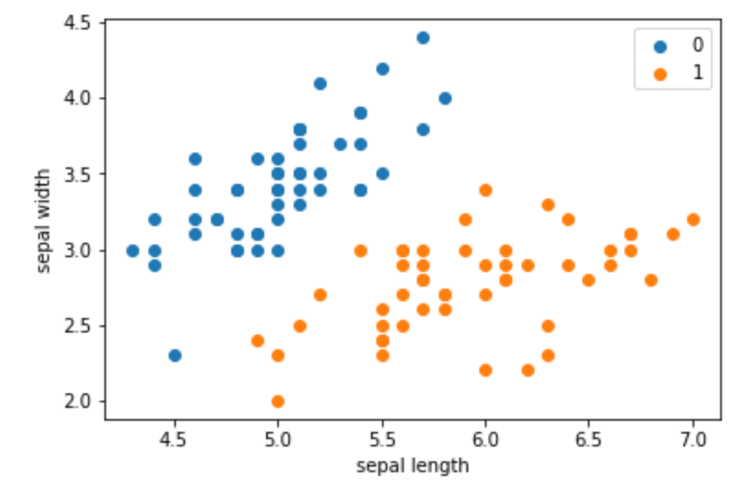
本部分将以iris数据集中的sepal length和sepal width作为特征，以iris的类别作为label，展示感知机算法的实现情况。

调用库

import pandas as pd
import numpy as np
from sklearn.datasets import load_iris
import matplotlib.pyplot as plt

加载数据集

iris = load_iris()
df = pd.DataFrame(iris.data, columns=iris.feature_names)
df['label'] = iris.target
df.columns = ['sepal length', 'sepal width', 'petal length', 'petal width', 'label']
df.label.value_counts()
data = np.array(df.iloc[:100, [0, 1, -1]])
X, y = data[:,:-1], data[:,-1]
y = np.array([1 if i == 1 else -1 for i in y])

数据可视化

plt.scatter(df[:50]['sepal length'], df[:50]['sepal width'], label='0')
plt.scatter(df[50:100]['sepal length'], df[50:100]['sepal width'], label='1')
plt.xlabel('sepal length')
plt.ylabel('sepal width')
plt.legend()
plt.show()

根据原始算法实现感知机模型

class Model:
    def __init__(self):
        self.w = np.ones(len(data[0]) - 1, dtype=np.float32)
        self.b = 0
        self.l_rate = 0.1
        # self.data = data

    def sign(self, x, w, b):
        y = np.dot(x, w) + b
        return y

    # 随机梯度下降法
    def fit(self, X_train, y_train):
        is_wrong = False
        while not is_wrong:
            wrong_count = 0  # 误分类点的个数
            for d in range(len(X_train)):
                X = X_train[d]
                y = y_train[d]
                if y * self.sign(X, self.w, self.b) <= 0:
                    self.w = self.w + self.l_rate * np.dot(y, X)
                    self.b = self.b + self.l_rate * y
                    wrong_count += 1
            if wrong_count == 0:
                is_wrong = True
        return 'Perceptron Model!'

利用原始算法拟合数据

perceptron = Model()
perceptron.fit(X, y)

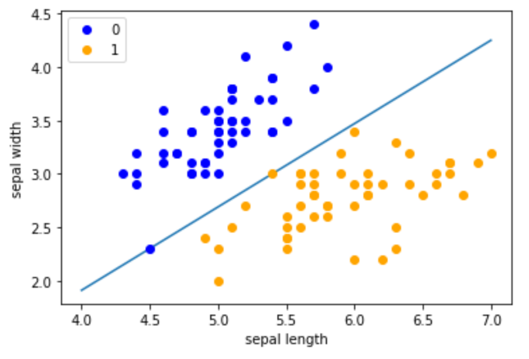
绘制原始算法分类效果图

x_points = np.linspace(4, 7, 10)
y_ = -(perceptron.w[0] * x_points + perceptron.b) / perceptron.w[1]
plt.plot(x_points, y_)

plt.plot(data[:50, 0], data[:50, 1], 'bo', color='blue', label='0')
plt.plot(data[50:100, 0], data[50:100, 1], 'bo', color='orange', label='1')
plt.xlabel('sepal length')
plt.ylabel('sepal width')
plt.legend()
plt.legend()
plt.show()

根据对偶算法实现感知机模型

class Perceptron:
    
    """Dual learning algorithm of perception"""
    
    def __init__(self, x):
        self.a = np.ones(len(x), dtype = np.float32)
        self.b = 1
        self.l_rate = 0.2
        self.Gram = np.dot(x, x.T)
        
    def sign(self, y, d):
        coef = np.multiply(self.a, y)
        sum1 = np.dot(coef, self.Gram[d]) + self.b
        return sum1
        
    def fit(self, X_train, y_train):
        is_wrong = False
        while not is_wrong:
            wrong_count = 0
            for i in range(len(X_train)):
                X = X_train
                y = y_train
                if y[i] * self.sign(y, i) <= 0:
                    self.a[i] += self.l_rate
                    self.b += self.l_rate * y[i]
                    wrong_count += 1
            if wrong_count == 0:
                is_wrong = True
        return 'Perceptron Model!'
    
    def score(self):
        pass

利用对偶算法拟合模型

perceptron = Perceptron(X)
perceptron.fit(X, y)

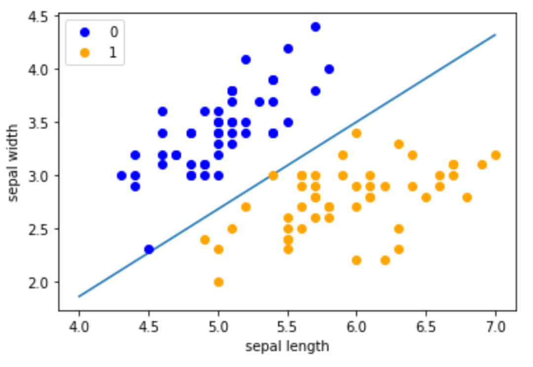
绘制原始算法分类效果图

x_points = np.linspace(4, 7, 10)
w = np.matmul(np.multiply(perceptron.a, y), X)
y_ = -(w[0] * x_points + perceptron.b) / w[1]
plt.plot(x_points, y_)
plt.plot(data[:50, 0], data[:50, 1], 'bo', color='blue', label='0')
plt.plot(data[50:100, 0], data[50:100, 1], 'bo', color='orange', label='1')
plt.xlabel('sepal length')
plt.ylabel('sepal width')
plt.legend()
plt.legend()
plt.show()