时间序列预测Python实现

数苗铺子 2021-05-19

1590

点击蓝字

默默关注

时间序列简单的说就是各时间点上形成的数值序列，时间序列分析就是通过观察历史数据预测未来的值。

时间序列分析并不是关于时间的回归，它主要是研究自身的变化规律的（这里不考虑含外生变量的时间序列）

本文所考虑的时间序列预测是只含根据序列本身来预测，不含其他内生或外生变量，且不分析序列的随机性，只关注预测部分（特别是SARIMA的Python实现）

预测评估指标

[R squared]：R²定系数（在计量经济学中，它可以理解为描述模型方差的百分比），描述模型的泛化能力，取值区间（-inf，1）为1时模型的性能最好。
链接：(http://scikit-learn.org/stable/modules/model_evaluation.html#r2-score-the-coefficient-of-determination)
[Mean Absolute Error]：平均绝对值损失，一种预测值与真实值之间的度量标准，也称作L1-norm损失，取值区间[0，inf)。
链接：(https://scikit-learn.org/stable/modules/model_evaluation.html#mean-absolute-error)
[Mean Absolute Percentage Error]：作用和MAE一样，只不过是以百分比的形式，用来解释模型的质量，但是在sklearn的库中，没有提供这个函数的接口，取值区间[0，inf)。
[Median Absolute Error]：绝对值损失的中位数，抗干扰能力强，对于有异常点的数据集的鲁棒性比较好，取值区间[0，inf)。
链接：(https://scikit-learn.org/stable/modules/model_evaluation.html#median-absolute-error)
[Mean Squared Error]：均方差损失，对于真实值与预测值偏差较大的样本点给予更高（平方）的惩罚，反之亦然，取值区间[0，inf)。
链接：(https://scikit-learn.org/stable/modules/model_evaluation.html#mean-squared-error)
[Mean squared logarithmic error]：均方对数误差，定义形式特别像上面提的MSE，只是计算的是真实值的自然对数与预测值的自然对数之差的平方，通常适用于 target 有指数的趋势时，取值区间[0，inf)。
链接：(https://scikit-learn.org/stable/modules/model_evaluation.html#mean-squared-logarithmic-error)

六类损失函数

from sklearn.metrics import r2_score,median_absolute_error,median_absolute_error, mean_squared_error, mean_squared_log_error

def mean_absolute_percentage_error(y_true, y_pred): 
    return np.mean(np.abs((y_true - y_pred) / y_true)) * 100

数据集

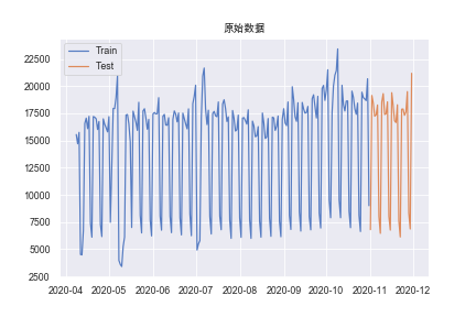
选择2021年招商银行FinTech比赛中业务A从2020年4月8日到2020年11月3-日的日数据，共237条。比赛中也给了一些其他的X变量，但在A，B榜中使用只用到y信息的SARIMA的模型会比使用X信息的LightGBM准确度高出30%左右（二者在极限调参与后者极限扩特征的情况下）

数据载入与前期处理


## 图像基本格式设置
import seaborn as sns
import matplotlib.pyplot as plt
plt.rcParams["font.family"] = 'Arial Unicode MS'
sns.set(context='paper',
        style='darkgrid',
        palette=sns.color_palette('muted',desat=0.8),
        color_codes=False) 

import numpy as np
import pandas as pd
from sklearn.metrics import mean_squared_error

def mape(y_true, y_pred):
    return np.mean(np.abs((y_pred - y_true) / (y_true+1)))

data = np.array([15554, 14701, 15751,  4517,  4478,  6724, 16566, 17065, 16095,
       17227,  7391,  6107, 17210, 17139, 16996, 16015, 16752,  7290,
        6162, 16994, 16498, 16169, 15797, 17199,  7478, 12575, 17952,
       17944, 18979, 20959,  3970,  3598,  3409,  5242,  6122, 17349,
       17395, 16541, 14861,  6997, 17705, 17170, 16679, 15936, 18519,
        8121,  6497, 17725, 17925, 17083, 16044, 16948,  7713,  6223,
       17442, 17582, 17441, 17481, 18942,  8061,  6751, 17236, 17407,
       16425, 16413, 17100,  8049,  6523, 16941, 17725, 17428, 16715,
       17538,  7898,  6316, 17521, 17023, 16531, 16078, 17914,  8237,
        6241, 18389, 19068, 20089,  4923,  5489,  5788, 17109, 20933,
       21670, 17938, 16471, 17791,  7993,  6400, 17480, 17682, 17279,
       17195, 18552,  8045,  6790, 18354, 18750, 17964, 16756, 17177,
        7707,  5998, 17765, 17052, 15870, 15996, 17338,  7887,  6089,
       17066, 17104, 16830, 16513, 17826,  7727,  5995, 16789, 16356,
       15351, 15425, 16280,  7593,  6104, 17531, 16597, 15197, 15308,
       17022,  7860,  6182, 17146, 17088, 15930, 16306, 17255,  7590,
        6149, 16951, 17929, 16616, 16374, 18548,  8092,  6816, 19953,
       18781, 17184, 16767, 18480,  8439,  6666, 18504, 17911, 17516,
       17584, 18139,  7991,  6780, 18843, 19210, 18095, 17076, 19068,
        8325,  6950, 19787, 20073, 18695, 19640, 21512,  9526,  7894,
       17551, 23045, 24015, 25430, 25430,  9526,  7894, 20086, 18310,
       17719, 18628, 18643,  8482,  6980, 19546, 18993, 17937, 17413,
       18443,  8100,  6629, 19449, 18952, 18830, 18675, 20686,  9005,
       6799., 19145., 18435., 17237., 17360., 18270,  8002,  6461,
       18528., 19316., 17397., 17467., 18560.,  8021.,  6759., 19403.,
       18223., 16814., 16655., 18291.,  7614.,  6127., 17882., 17899.,
       17318., 17632., 19503.,  8332.,  6860., 21184.])



# 生成时间索引
data = pd.DataFrame({'date':pd.date_range('2020-04-08','2020-11-30',freq='D'),'amount':data})
data.index = data.date # 将字符串索引转换成时间索引

# 划分训练集与测试集
train = data[:-30]
test = data[-30:]

# 展示序列
plt.rcParams["font.family"] = 'Arial Unicode MS'
plt.plot(train.index, train['amount'], label='Train')
plt.plot(test.index,test['amount'], label='Test')
plt.legend()
plt.title('原始数据')
plt.show()

平稳性检验

时间序列的平稳性是时间序列分析过程中进行许多统计操作处理的基本前提假设。所以，非平稳的时间序列数据常常需要被转换成平稳性的数据。时间序列的平稳性过程是一个随机过程，它的无条件联合概率分布不会随着时间的变换而变换，所以平稳序列的均值和方差等参数也不会随时间的变化而变化，这就为后续的平稳性检验提供理论基础。

检验方法

查看时间序列图：从原始数据图中可见有明显的季节因素，时间序列不平稳，无法判断是否有长期趋势。

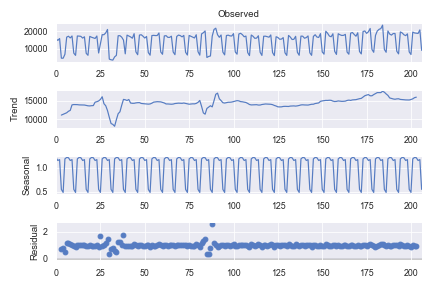
时间序列分解：提取序列的趋势、季节和随机效应。对于非平稳的时间序列，可以通过对趋势和季节性进行建模并将它们从模型中剔除，从而将非平稳的数据转换为平稳数据，并对其残差进行进一步的分析。

经典的时间序列分解并提取各类序列

from statsmodels.tsa.seasonal import seasonal_decompose
# 设置为加法模型，period为季节长度
result = seasonal_decompose(np.array(train['amount']), 
                            model='multiplicative', period=7)

result.plot()
plt.show()

## 提取各类效应序列
trend = result.trend #趋势效应
seasonal = result.seasonal #季节效应
residual = result.resid #随机效应

STL时间序列分解

from statsmodels.tsa.seasonal import STL
result = STL(np.array(train['amount']), period=7, robust=True)
result = result.fit()
result.plot()
plt.show()

绘制移动平均值和标准差

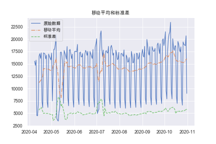
一种正式的方法是绘制移动平均值和标准差，通过观察时间序列的平均值和标准差是否随时间变化来判断序列是否平稳。.rolling(window = 12, center = False)

rol_mean = train['amount'].rolling(window = 7, center = False).mean()
rol_std = train['amount'].rolling(window = 7, center = False).std()

plt.plot(train['amount'],label = u'原始数据')
plt.plot(rol_mean, linestyle='-.', label = u'移动平均')
plt.plot(rol_std, linestyle='--', label = u'标准差')

plt.legend(loc='best')
plt.title(u'移动平均和标准差')
plt.show(block= True)

ADF检验

检验的零假设是时间序列是非平稳的。检验结果比较了不同置信水平下的检验统计量和临界值。如果“检验统计量”小于“临界值”，我们可以拒绝零假设，认为在给定的显著性水平下这个序列是平稳的。

from statsmodels.tsa.stattools import adfuller
def TestStationaryAdfuller(ts, cutoff = 0.01):
    ts_test = adfuller(ts, autolag = 'AIC')
    ts_test_output = pd.Series(ts_test[0:4], index=['Test Statistic','p-value','#Lags Used','Number of Observations Used'])

    for key,value in ts_test[4].items():
        ts_test_output['Critical Value (%s)'%key] = value
    print(ts_test_output)

    if ts_test[1] <= cutoff:
        print(u"拒绝原假设，即数据没有单位根,序列是平稳的。")
    else:
        print(u"不能拒绝原假设，即数据存在单位根,数据是非平稳序列。")
  
TestStationaryAdfuller(train['amount'])

序列平稳化

消除时间序列的趋势效应和季节性效应最常用方法之一是差分法。对原始的序列作1阶7步差分来提取原序列的趋势效应和季节效应。

Note:这里关于季节和趋势差分的选择以及先后顺序都需多多尝试，一般二者阶数不会太高

#消除消除趋势和季节性
train_first_difference = train['amount'] - train['amount'].shift(1) #一阶差分
train_seasonal_first_difference = train_first_difference - train_first_difference.shift(12) #12步差分
TestStationaryAdfuller(train_first_difference.dropna(inplace=False))
TestStationaryAdfuller(train_seasonal_first_difference.dropna(inplace=False))

白噪声检验

当序列平稳之后，对序列需要进行白噪声检验，如果序列是白噪声序列，则序列中没有信息可以提取，不需要再做模型，反之可以做AR、MA等模型。

#白噪声检验
import statsmodels.api as sm
train_seasonal_first_difference.dropna(inplace = True)
r,q,p = sm.tsa.acf(train_seasonal_first_difference.values.squeeze(), qstat=True) 
data = np.c_[range(1,41), r[1:], q, p] 
table = pd.DataFrame(data, columns=['lag', "AC", "Q", "Prob(>Q)"]) 
print(table.set_index('lag'))

SARIMA模型

模型定阶

两种方法来进行模型定阶，其中需要定阶的参数有7个，包含趋势项的差分阶数，AR和MA阶数与季节项的上述是那个参数和季节步数。

自相关与偏自相关图识别：

#寻找最优参数，建立SARIMA模型
fig = plt.figure(figsize=(12,8))
ax1 = fig.add_subplot(211)
fig = sm.graphics.tsa.plot_acf(train_seasonal_first_difference, lags=40, ax=ax1)
ax2 = fig.add_subplot(212)
fig = sm.graphics.tsa.plot_pacf(train_seasonal_first_difference, lags=40, ax=ax2)
plt.show()

从图中看，考虑1阶7步差分后的序列7阶以内自相关系数和偏自相关系数的特征，发现自相关图和偏自相关图显示7阶以内自相关系数和偏自相关系数均是拖尾，所以尝试使用ARMA（1，1）再考虑季节自相关和偏自相关特征，观察延迟7阶、14阶等以周期长度为单位的自相关系数和偏自相关系数的特征。

可以发现，二者均拖尾。可以考虑以7步为周期的ARMA（1，1）7中（1，1）以上的模型提取差分后序列的季节自相关和偏自相关信息。

直接拟合SARIMA模型，网格搜索，通过AIC等准则选取最优模型。

用图解法求解ARIMA模型的最优参数并非易事，主观性很大，而且耗费时间。所以进一步考虑利用网格搜索的方法系统地选择最优的参数值。当网格搜索遍历完整个参数环境是，我们可以依据评价时间序列模型的准则从参数集中选出最佳性能的参数。

在评估和比较具有不同参数的统计模型时，可以根据数据的拟合程度或准确预测未来数据点的能力对每个模型进行排序。本文考虑使用AIC准则来评价选取模型。AIC准则是拟合精度和参数个数的加权函数，使AIC函数达到最小的模型被认为是最优模型

import itertools
p = d = q = range(1, 3) 
pdq = list(itertools.product(p, d, q)) 
pdq_x_PDQs = [(x[0], x[1], x[2], 7) for x in list(itertools.product(p, d, q))] 
a=[]
b=[]
c=[]
wf=pd.DataFrame()
for param in pdq:
    for seasonal_param in pdq_x_PDQs:
        try:
            mod = sm.tsa.statespace.SARIMAX(np.array(train['amount']),order=param,seasonal_order=seasonal_param,enforce_stationarity=False,enforce_invertibility=False)
            results = mod.fit()
            print('ARIMA{}x{} - AIC:{}'.format(param, seasonal_param, results.aic))
            a.append(param)
            b.append(seasonal_param)
            c.append(results.aic)
        except:
            continue
wf['pdq']=a
wf['pdq_x_PDQs']=b
wf['aic']=c
print(wf[wf['aic']==wf['aic'].min()])

输出为（1，1，1）（2，2，2，7）

模型建立

拟合

model = sm.tsa.statespace.SARIMAX(np.array(train['amount']), 
                                order=(1,1,1), 
                                seasonal_order=(2,2,2,7),   
                                enforce_stationarity=False,
                                enforce_invertibility=False)
results = model.fit()
print(results.summary())

若变量的P值小于0.01，则在0.01的显著性水平下，拒绝原假设，该变量的通过显著性检验，否则可考虑去掉该变量或检查模型。

模型检验

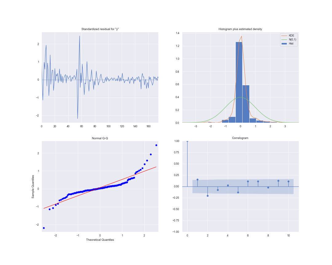
在拟合SARIMA模型时，模型诊断是非常重要的一步，通过模型诊断以确保模型所做的任何假设都没有被违反。

模型检验中我们主要关心的问题是模型的残差是否相关的，并且是否是零均值的正态分布。如果SARIMA模型残差是相关的，且不是零均值正态分布，则表明模型可以进一步改进，反之，模型拟合效果很好，可以认为模型充分提取了序列的信息。

对于残差白噪声的检验，采用LB检验的方法对模型的残差是否为白噪声序列进行检验。

对于残差的分布问题，Python中的plot_diagnostic函数可以快速生成模型诊断并研究模型的异常行为。

#模型检验
#模型诊断
results.plot_diagnostics(figsize=(15, 12))
plt.show()
#LB检验
r,q,p = sm.tsa.acf(results.resid.squeeze(), qstat=True) 
data = np.c_[range(1,41), r[1:], q, p] 
table = pd.DataFrame(data, columns=['lag', "AC", "Q", "Prob(>Q)"]) 
print(table.set_index('lag'))

lag	AC	Q	Prob(>Q)
1	-0.14	4.48	0.03
2	-0.25	18.1	<0.01
3	-0.02	18.2	<0.01
4	0.08	19.6	<0.01
5	-0.21	29.9	<0.01
6	0.24	43.0	<0.01
7	0.05	43.6	<0.01

由上图的模型诊断结果可知，残差的的时序图并不稳定，残差并不是随机正态分布，还有信息可以提取，但自相关图显示序列不相关了，后续可考虑建模，这里不再对残差进行建模了。

由上表可见，残差序列延迟1-7阶时，Q统计量的P值均小于0.05，所以在0.05的显著性水平下，拒绝原假设，即残差为不为白噪声序列，与图结果相符。

（但这里不再对残差进行建模了，若只追求拟合效果，其实这个也不是很重要）

模型预测

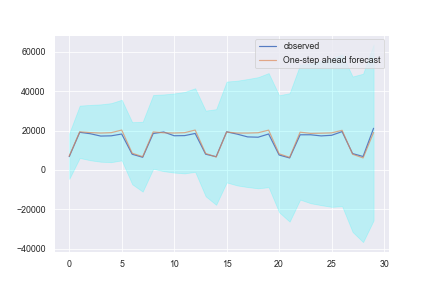
直接选取整个测试集进行预测（这里测试集选用的是最后的30天）

pred = results.get_prediction(start = len(train) ,end = len(train)+len(test)-1, dynamic=False)
pred_ci = pd.DataFrame(pred.conf_int())
test_forecast = pd.Series(pred.predicted_mean)
test_true = pd.Series(np.array(test['amount']))
test_pred_concat = pd.concat([test_true, test_forecast,pred_ci],axis=1)
test_pred_concat.columns = [u'原始值',u'预测值',u'下限',u'上限']
test_pred_concat.head(30)

ax = test_true.plot(label='observed')
test_forecast.plot(ax=ax, label='One-step ahead forecast', alpha=.7)
ax.fill_between(pred_ci.index,pred_ci.iloc[:,0],pred_ci.iloc[:,1], color='cyan', alpha=.2)
plt.legend()
plt.savefig('png12.png')
plt.show()

print('MAPE:',mape(np.array(test_pred_concat['原始值']),np.array(test_pred_concat['预测值'])))
print('MSE:',mean_squared_error(np.array(test_pred_concat['原始值']),np.array(test_pred_concat['预测值'])))

其他时间序列预测方法

移动平均 (Moving Average)

假设未来某个值的预测，取决于它前面的 n 个数的平均值，因此，我们将用 moving average (移动平均数) 作为 target 的预测值，表达式为：

def average(Y, h):
    """
        Calculate average of last n observations
    """
    return np.mean(Y[-h:])

def moving_average(Y,h,n):
    """
    Y:时间序列数据
    h:用前h的数据移动平均预测
    n:向后预测n个数据
    RETURN:
    Y_pre:预测数据

    """
    Y_pre = np.array(Y)
    for i in range(n):
        Y_pre = np.append(Y_pre,average(Y_pre,h)) 
    return Y_pre[-n:] 
        
pre = moving_average(train['amount'],30,30) 

print('MAPE:',mape(test['amount'],pre))
print('MSE:',mean_squared_error(test['amount'],pre))

plt.rcParams["font.family"] = 'Arial Unicode MS'
plt.plot(train.index, train['amount'], label='Train')
plt.plot(test.index,test['amount'], label='Test')
plt.plot(test.index,pre, label='Prediction')
plt.legend()
plt.title('Moving Average预测')
plt.show()

==Problem==:上面这种方式，不适合我们进行长期的预测（为了预测下一个值，我们需要实际观察的上一个值）。

但是 移动平均数 还有另一个应用场景，即对原始的时间序列数据进行平滑处理，以找到数据的变化趋势。

加权平均值(Weighted Average)

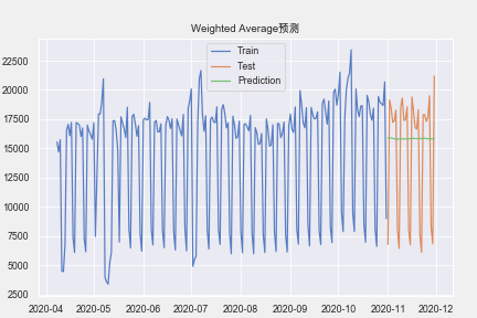
前面h个观测数据的值，不再是直接求和再取平均值，而是计算它们的加权和（权重和为1）。通常来说，时间距离越近的观测点，权重越大。数学表达式为：

weights = np.arange(30)/sum(np.arange(30)) # 生成一种weights

def weighted_average(Y, weights):
    """
        Calculate weighter average on series
    """
    h = len(weights)
    return np.dot(Y[-h:],weights)


def moving_weighted_average(Y,weights,n):
    """
    Y:时间序列数据
    h:用前h的数据移动平均预测
    n:向后预测n个数据
    RETURN:
    Y_pre:预测数据

    """
    Y_pre = np.array(Y)
    for i in range(n):
        Y_pre = np.append(Y_pre,weighted_average(Y_pre,weights)) 
    return Y_pre[-n:] 
        
pre = moving_weighted_average(train['amount'],weights,30)  # 预测
  
print('MAPE:',mape(test['amount'],pre))
print('MSE:',mean_squared_error(test['amount'],pre))

plt.rcParams["font.family"] = 'Arial Unicode MS'
plt.plot(train.index, train['amount'], label='Train')
plt.plot(test.index,test['amount'], label='Test')
plt.plot(test.index,pre, label='Prediction')
plt.legend()
plt.title('Weighted Average预测')
plt.savefig('png3.png')
plt.show()

Image

指数平滑(Exponential Smoothing)

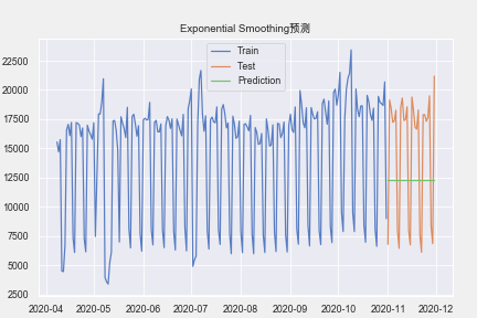
直接对目前所有的已观测数据进行加权处理，并且每一个数据点的权重，呈指数形式递减。

:平滑因子, 越小，表示当前观测值的影响力越小

代码

statsmodels.tsa.api.SimpleExpSmoothing

import statsmodels.tsa.api as tsa
# np.array(train['amount'])之后时间索引变成了1-len(train)的数值
model = tsa.SimpleExpSmoothing(np.array(train['amount']), 
                               initialization_method="estimated")
#smoothing_level为alpha
model.fit(smoothing_level=0.7,optimized=False) 
# 注意下面这个预测方法
pre = model.predict(params=model.params,start=len(train),end=len(train)+29)

print('MSE:',mape(test['amount'],pre))
print('MAPE:',mean_squared_error(test['amount'],pre))

plt.rcParams["font.family"] = 'Arial Unicode MS'
plt.plot(train.index, train['amount'], label='Train')
plt.plot(test.index,test['amount'], label='Test')
plt.plot(test.index,pre,label='Prediction')
plt.legend()
plt.title('Exponential Smoothing预测')
plt.show()

Holt-Winters三参数指数平滑

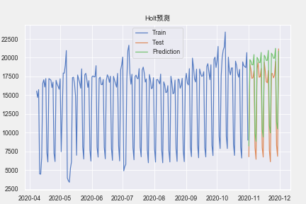
假设要进行指数平滑的序列为,序列既含有趋势又含有季节若季节和趋势是加法模型，则有

若乘法则有

:该序列的水平部分
:为该序列的趋势部分
:为该序列的季节因子（假设季节周期长度为）

在python中均可自动给出

我们从图中可以看出，该数据集没啥趋势。但为展示代码，还是用加法的Holt-Winters，预测未来价格。

import statsmodels.tsa.api as tsa
model = tsa.ExponentialSmoothing(np.array(train['amount']), seasonal_periods=7, 
                                 trend='add', seasonal='add',
                                 initialization_method="estimated").fit(use_boxcox=True)
pre = model.forecast(30)
  
print('MAPE:',mape(test['amount'],pre))
print('MSE:',mean_squared_error(test['amount'],pre))

plt.rcParams["font.family"] = 'Arial Unicode MS'
plt.plot(train.index, train['amount'], label='Train')
plt.plot(test.index,test['amount'], label='Test')
plt.plot(test.index,pre,label='Prediction')
plt.legend()
plt.title('Holt预测')
plt.show()

SARIMA

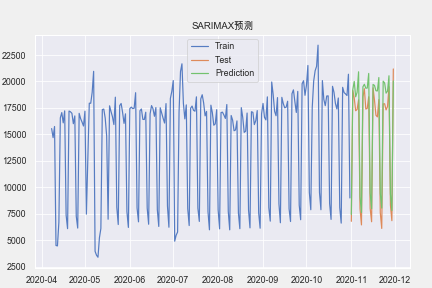
import statsmodels.api as sm
model = sm.tsa.statespace.SARIMAX(np.array(train['amount']), order=(4, 1, 4), seasonal_order=(0, 1, 2, 7)).fit()
pre = model.predict(start=len(train),end=len(train)+59, dynamic=True)

print('MSE:',mape(test['amount'],pre))
print('MAPE:',mean_squared_error(test['amount'],pre))

plt.rcParams["font.family"] = 'Arial Unicode MS'
plt.plot(train.index, train['amount'], label='Train')
plt.plot(test.index,test['amount'], label='Test')
plt.plot(test.index,pre,label='Prediction')
plt.legend()
plt.title('SARIMAX预测')
plt.show()

参考资料

[1]关于SARIMA完整的例子https://zhuanlan.zhihu.com/p/127032260

[2]Statsmodel库：https://www.statsmodels.org/stable/api.html

[3]关于时间序列预测的7种方法：https://www.cnblogs.com/lfri/p/12243268.html

喜欢就关注我吧，订阅更多最新消息

python

文章转载自数苗铺子，如果涉嫌侵权，请发送邮件至：contact@modb.pro进行举报，并提供相关证据，一经查实，墨天轮将立刻删除相关内容。

时间序列预测Python实现

代码

参考资料

评论