


1、导入模块
 1import numpy as np
 2from netCDF4 import Dataset
 3import matplotlib.pyplot as plt
 4from matplotlib.cm import get_cmap
 5from matplotlib.colors import from_levels_and_colors
 6import cartopy.crs as crs
 7import cartopy.feature as cfeature
 8from cartopy.feature import NaturalEarthFeature
 9from wrf import to_np, getvar, interplevel, smooth2d, get_cartopy, cartopy_xlim, cartopy_ylim, latlon_coords, vertcross, smooth2d, CoordPair, GeoBounds,interpline
10
11import warnings
12warnings.filterwarnings('ignore')
2、读取数据
1wrf_file = '../input/wrf3880/wrfout_d01_2016-10-07_00_00_00_subset.nc'
2# Open the NetCDF file
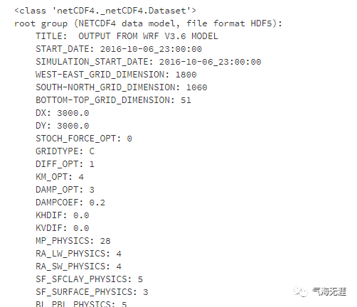
3ncfile = Dataset(wrf_file)
4ncfile
3、绘制海平面气压场
 1# Get the sea level pressure
 2slp = getvar(ncfile, "slp")
 3
 4# Smooth the sea level pressure since it tends to be noisy near the
 5# mountains
 6smooth_slp = smooth2d(slp, 3, cenweight=4)
 7
 8# Get the latitude and longitude points
 9lats, lons = latlon_coords(slp)
10
11# Get the cartopy mapping object
12cart_proj = get_cartopy(slp)
13
14# Create a figure
15fig = plt.figure(figsize=(12,6))
16# Set the GeoAxes to the projection used by WRF
17ax = plt.axes(projection=cart_proj)
18
19# Download and add the states and coastlines
20states = NaturalEarthFeature(category="cultural", scale="50m",
21                             facecolor="none",
22                             name="admin_1_states_provinces_shp")
23ax.add_feature(states, linewidth=.5, edgecolor="black")
24ax.coastlines('50m', linewidth=0.8)
25
26# Make the contour outlines and filled contours for the smoothed sea level
27# pressure.
28plt.contour(to_np(lons), to_np(lats), to_np(smooth_slp), 10, colors="black",
29            transform=crs.PlateCarree())
30plt.contourf(to_np(lons), to_np(lats), to_np(smooth_slp), 10,
31             transform=crs.PlateCarree(),
32             cmap=get_cmap("jet"))
33
34# Add a color bar
35plt.colorbar(ax=ax, shrink=.98)
36
37# Set the map bounds
38ax.set_xlim(cartopy_xlim(smooth_slp))
39ax.set_ylim(cartopy_ylim(smooth_slp))
40
41# Add the gridlines
42ax.gridlines(color="black", linestyle="dotted")
43
44plt.title("Sea Level Pressure (hPa)")
45plt.show()

4、绘制500hPa位视高度和风场
1# Extract the pressure, geopotential height, and wind variables
2p = getvar(ncfile, "pressure")
3z = getvar(ncfile, "z", units="dm")
4ua = getvar(ncfile, "ua", units="kt")
5va = getvar(ncfile, "va", units="kt")
6wspd = getvar(ncfile, "wspd_wdir", units="kts")[0,:]
7
8# Interpolate geopotential height, u, and v winds to 500 hPa
9ht_500 = interplevel(z, p, 500)
10u_500 = interplevel(ua, p, 500)
11v_500 = interplevel(va, p, 500)
12wspd_500 = interplevel(wspd, p, 500)
13
14# Get the lat/lon coordinates
15lats, lons = latlon_coords(ht_500)
16
17# Get the map projection information
18cart_proj = get_cartopy(ht_500)
19
20# Create the figure
21fig = plt.figure(figsize=(12,9))
22ax = plt.axes(projection=cart_proj)
23
24# Download and add the states and coastlines
25states = NaturalEarthFeature(category="cultural", scale="50m",
26 facecolor="none",
27 name="admin_1_states_provinces_shp")
28ax.add_feature(states, linewidth=0.5, edgecolor="black")
29ax.coastlines('50m', linewidth=0.8)
30
31# Add the 500 hPa geopotential height contours
32levels = np.arange(520., 580., 6.)
33contours = plt.contour(to_np(lons), to_np(lats), to_np(ht_500),
34 levels=levels, colors="black",
35 transform=crs.PlateCarree())
36plt.clabel(contours, inline=1, fontsize=10, fmt="%i")
37
38# Add the wind speed contours
39levels = [25, 30, 35, 40, 50, 60, 70, 80, 90, 100, 110, 120]
40wspd_contours = plt.contourf(to_np(lons), to_np(lats), to_np(wspd_500),
41 levels=levels,
42 cmap=get_cmap("rainbow"),
43 transform=crs.PlateCarree())
44plt.colorbar(wspd_contours, ax=ax, orientation="horizontal", pad=.05)
45
46# Add the 500 hPa wind barbs, only plotting every 125th data point.
47plt.barbs(to_np(lons[::125,::125]), to_np(lats[::125,::125]),
48 to_np(u_500[::125, ::125]), to_np(v_500[::125, ::125]),
49 transform=crs.PlateCarree(), length=6)
50# Set the map bounds
51ax.set_xlim(cartopy_xlim(ht_500))
52ax.set_ylim(cartopy_ylim(ht_500))
53ax.gridlines()
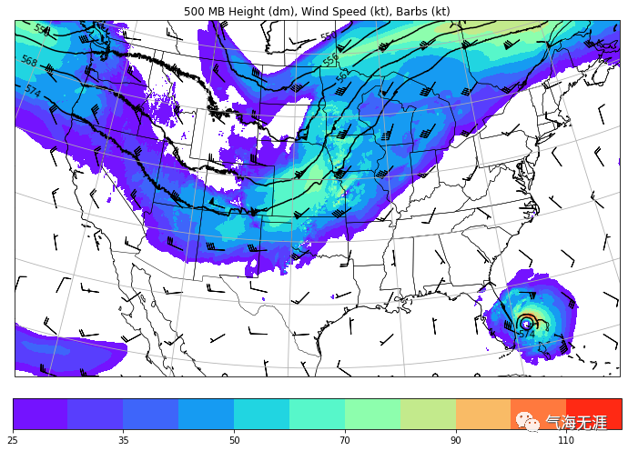
54plt.title("500 MB Height (dm), Wind Speed (kt), Barbs (kt)")
55plt.show()
5、绘制经向剖面图
1# Get the WRF variables
2slp = getvar(ncfile, "slp")
3smooth_slp = smooth2d(slp, 3)
4ctt = getvar(ncfile, "ctt")
5z = getvar(ncfile, "z")
6dbz = getvar(ncfile, "dbz")
7Z = 10**(dbz/10.)
8wspd = getvar(ncfile, "wspd_wdir", units="kt")[0,:]
9
10# Set the start point and end point for the cross section
11start_point = CoordPair(lat=26.76, lon=-80.0)
12end_point = CoordPair(lat=26.76, lon=-77.8)
13
14# Compute the vertical cross-section interpolation. Also, include the
15# lat/lon points along the cross-section in the metadata by setting latlon
16# to True.
17z_cross = vertcross(Z, z, wrfin=ncfile, start_point=start_point,
18 end_point=end_point, latlon=True, meta=True)
19wspd_cross = vertcross(wspd, z, wrfin=ncfile, start_point=start_point,
20 end_point=end_point, latlon=True, meta=True)
21dbz_cross = 10.0 * np.log10(z_cross)
22
23# Get the lat/lon points
24lats, lons = latlon_coords(slp)
25
26# Get the cartopy projection object
27cart_proj = get_cartopy(slp)
28
29# Create a figure that will have 3 subplots
30fig = plt.figure(figsize=(12,9))
31ax_ctt = fig.add_subplot(1,2,1,projection=cart_proj)
32ax_wspd = fig.add_subplot(2,2,2)
33ax_dbz = fig.add_subplot(2,2,4)
34
35# Download and create the states, land, and oceans using cartopy features
36states = cfeature.NaturalEarthFeature(category='cultural', scale='50m',
37 facecolor='none',
38 name='admin_1_states_provinces_shp')
39land = cfeature.NaturalEarthFeature(category='physical', name='land',
40 scale='50m',
41 facecolor=cfeature.COLORS['land'])
42ocean = cfeature.NaturalEarthFeature(category='physical', name='ocean',
43 scale='50m',
44 facecolor=cfeature.COLORS['water'])
45
46# Make the pressure contours
47contour_levels = [960, 965, 970, 975, 980, 990]
48c1 = ax_ctt.contour(lons, lats, to_np(smooth_slp), levels=contour_levels,
49 colors="white", transform=crs.PlateCarree(), zorder=3,
50 linewidths=1.0)
51
52# Create the filled cloud top temperature contours
53contour_levels = [-80.0, -70.0, -60, -50, -40, -30, -20, -10, 0, 10]
54ctt_contours = ax_ctt.contourf(to_np(lons), to_np(lats), to_np(ctt),
55 contour_levels, cmap=get_cmap("Greys"),
56 transform=crs.PlateCarree(), zorder=2)
57
58ax_ctt.plot([start_point.lon, end_point.lon],
59 [start_point.lat, end_point.lat], color="yellow", marker="o",
60 transform=crs.PlateCarree(), zorder=3)
61
62# Create the color bar for cloud top temperature
63cb_ctt = fig.colorbar(ctt_contours, ax=ax_ctt, shrink=.60)
64cb_ctt.ax.tick_params(labelsize=5)
65
66# Draw the oceans, land, and states
67ax_ctt.add_feature(ocean)
68ax_ctt.add_feature(land)
69ax_ctt.add_feature(states, linewidth=.5, edgecolor="black")
70
71# Crop the domain to the region around the hurricane
72hur_bounds = GeoBounds(CoordPair(lat=np.amin(to_np(lats)), lon=-85.0),
73 CoordPair(lat=30.0, lon=-72.0))
74ax_ctt.set_xlim(cartopy_xlim(ctt, geobounds=hur_bounds))
75ax_ctt.set_ylim(cartopy_ylim(ctt, geobounds=hur_bounds))
76ax_ctt.gridlines(color="white", linestyle="dotted")
77
78# Make the contour plot for wind speed
79wspd_contours = ax_wspd.contourf(to_np(wspd_cross), cmap=get_cmap("jet"))
80# Add the color bar
81cb_wspd = fig.colorbar(wspd_contours, ax=ax_wspd)
82cb_wspd.ax.tick_params(labelsize=5)
83
84# Make the contour plot for dbz
85levels = [5 + 5*n for n in range(15)]
86dbz_contours = ax_dbz.contourf(to_np(dbz_cross), levels=levels,
87 cmap=get_cmap("jet"))
88cb_dbz = fig.colorbar(dbz_contours, ax=ax_dbz)
89cb_dbz.ax.tick_params(labelsize=5)
90
91# Set the x-ticks to use latitude and longitude labels
92coord_pairs = to_np(dbz_cross.coords["xy_loc"])
93x_ticks = np.arange(coord_pairs.shape[0])
94x_labels = [pair.latlon_str() for pair in to_np(coord_pairs)]
95ax_wspd.set_xticks(x_ticks[::20])
96ax_wspd.set_xticklabels([], rotation=45)
97ax_dbz.set_xticks(x_ticks[::20])
98ax_dbz.set_xticklabels(x_labels[::20], rotation=45, fontsize=4)
99
100# Set the y-ticks to be height
101vert_vals = to_np(dbz_cross.coords["vertical"])
102v_ticks = np.arange(vert_vals.shape[0])
103ax_wspd.set_yticks(v_ticks[::20])
104ax_wspd.set_yticklabels(vert_vals[::20], fontsize=4)
105ax_dbz.set_yticks(v_ticks[::20])
106ax_dbz.set_yticklabels(vert_vals[::20], fontsize=4)
107
108# Set the x-axis and y-axis labels
109ax_dbz.set_xlabel("Latitude, Longitude", fontsize=5)
110ax_wspd.set_ylabel("Height (m)", fontsize=5)
111ax_dbz.set_ylabel("Height (m)", fontsize=5)
112
113# Add a title
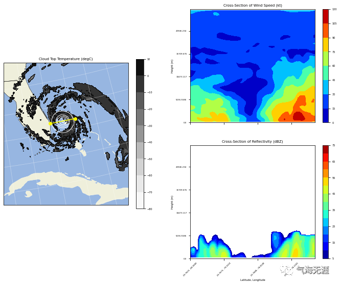
114ax_ctt.set_title("Cloud Top Temperature (degC)", {"fontsize" : 7})
115ax_wspd.set_title("Cross-Section of Wind Speed (kt)", {"fontsize" : 7})
116ax_dbz.set_title("Cross-Section of Reflectivity (dBZ)", {"fontsize" : 7})
117
118plt.show()
6、绘制山地的剖面图
  1# Define the cross section start and end points
  2cross_start = CoordPair(lat=43.5, lon=-116.5)
  3cross_end = CoordPair(lat=43.5, lon=-114)
  4
  5# Get the WRF variables
  6ht = getvar(ncfile, "z", timeidx=-1)
  7ter = getvar(ncfile, "ter", timeidx=-1)
  8dbz = getvar(ncfile, "dbz", timeidx=-1)
  9max_dbz = getvar(ncfile, "mdbz", timeidx=-1)
 10Z = 10**(dbz/10.) # Use linear Z for interpolation
 11
 12# Compute the vertical cross-section interpolation.  Also, include the
 13# lat/lon points along the cross-section in the metadata by setting latlon
 14# to True.
 15z_cross = vertcross(Z, ht, wrfin=ncfile,
 16                    start_point=cross_start,
 17                    end_point=cross_end,
 18                    latlon=True, meta=True)
 19
 20# Convert back to dBz after interpolation
 21dbz_cross = 10.0 * np.log10(z_cross)
 22
 23# Add back the attributes that xarray dropped from the operations above
 24dbz_cross.attrs.update(z_cross.attrs)
 25dbz_cross.attrs["description"] = "radar reflectivity cross section"
 26dbz_cross.attrs["units"] = "dBZ"
 27
 28# To remove the slight gap between the dbz contours and terrain due to the
 29# contouring of gridded data, a new vertical grid spacing, and model grid
 30# staggering, fill in the lower grid cells with the first non-missing value
 31# for each column.
 32
 33# Make a copy of the z cross data. Let's use regular numpy arrays for this.
 34dbz_cross_filled = np.ma.copy(to_np(dbz_cross))
 35
 36# For each cross section column, find the first index with non-missing
 37# values and copy these to the missing elements below.
 38for i in range(dbz_cross_filled.shape[-1]):
 39    column_vals = dbz_cross_filled[:,i]
 40    # Let's find the lowest index that isn't filled. The nonzero function
 41    # finds all unmasked values greater than 0. Since 0 is a valid value
 42    # for dBZ, let's change that threshold to be -200 dBZ instead.
 43    first_idx = int(np.transpose((column_vals > -200).nonzero())[0])
 44    dbz_cross_filled[0:first_idx, i] = dbz_cross_filled[first_idx, i]
 45
 46# Get the terrain heights along the cross section line
 47ter_line = interpline(ter, wrfin=ncfile, start_point=cross_start,end_point=cross_end)
 48
 49# Get the lat/lon points
 50lats, lons = latlon_coords(dbz)
 51
 52# Get the cartopy projection object
 53cart_proj = get_cartopy(dbz)
 54
 55# Create the figure
 56fig = plt.figure(figsize=(8,6))
 57ax_cross = plt.axes()
 58
 59dbz_levels = np.arange(5., 75., 5.)
 60
 61# Create the color table found on NWS pages.
 62dbz_rgb = np.array([[4,233,231],
 63                    [1,159,244], [3,0,244],
 64                    [2,253,2], [1,197,1],
 65                    [0,142,0], [253,248,2],
 66                    [229,188,0], [253,149,0],
 67                    [253,0,0], [212,0,0],
 68                    [188,0,0],[248,0,253],
 69                    [152,84,198]], np.float32) / 255.0
 70
 71dbz_map, dbz_norm = from_levels_and_colors(dbz_levels, dbz_rgb,extend="max")
 72
 73# Make the cross section plot for dbz
 74dbz_levels = np.arange(5.,75.,5.)
 75xs = np.arange(0, dbz_cross.shape[-1], 1)
 76ys = to_np(dbz_cross.coords["vertical"])
 77dbz_contours = ax_cross.contourf(xs,
 78                                 ys,
 79                                 to_np(dbz_cross_filled),
 80                                 levels=dbz_levels,
 81                                 cmap=dbz_map,
 82                                 norm=dbz_norm,
 83                                 extend="max")
 84# Add the color bar
 85cb_dbz = fig.colorbar(dbz_contours, ax=ax_cross)
 86cb_dbz.ax.tick_params(labelsize=8)
 87
 88# Fill in the mountain area
 89ht_fill = ax_cross.fill_between(xs, 0, to_np(ter_line),
 90                                facecolor="saddlebrown")
 91
 92# Set the x-ticks to use latitude and longitude labels
 93coord_pairs = to_np(dbz_cross.coords["xy_loc"])
 94x_ticks = np.arange(coord_pairs.shape[0])
 95x_labels = [pair.latlon_str() for pair in to_np(coord_pairs)]
 96
 97# Set the desired number of x ticks below
 98num_ticks = 5
 99thin = int((len(x_ticks) / num_ticks) + .5)
100ax_cross.set_xticks(x_ticks[::thin])
101ax_cross.set_xticklabels(x_labels[::thin], rotation=45, fontsize=8)
102
103# Set the x-axis and  y-axis labels
104ax_cross.set_xlabel("Latitude, Longitude", fontsize=12)
105ax_cross.set_ylabel("Height (m)", fontsize=12)
106
107# Add a title
108ax_cross.set_title("Cross-Section of Reflectivity (dBZ)", {"fontsize" : 14})
109plt.show()

有问题可以到QQ群里进行讨论,我们在那边等大家。
QQ群号:854684131
文章转载自气海无涯,如果涉嫌侵权,请发送邮件至:contact@modb.pro进行举报,并提供相关证据,一经查实,墨天轮将立刻删除相关内容。
