


1、导入模块
 1import numpy
 2import cartopy
 3from cartopy import crs
 4from cartopy.feature import NaturalEarthFeature, COLORS
 5import matplotlib.pyplot as plt
 6from matplotlib.cm import get_cmap
 7from matplotlib.colors import from_levels_and_colors
 8from netCDF4 import Dataset
 9from xarray import DataArray
10from wrf import getvar, interplevel, vertcross,vinterp, ALL_TIMES, CoordPair, xy_to_ll, ll_to_xy, to_np, get_cartopy, latlon_coords, cartopy_xlim, cartopy_ylim
11from matplotlib.animation import FuncAnimation
12from IPython.display import HTML
13import os
14import warnings
15warnings.filterwarnings('ignore')
2、读取文件
 1WRF_DIRECTORY = "../input/wrf3880"
 2WRF_FILES = ["wrfout_d01_2005-08-28_00_00_00",
 3             "wrfout_d01_2005-08-28_12_00_00",
 4             "wrfout_d01_2005-08-29_00_00_00"]
 5
 6_WRF_FILES = [os.path.abspath(os.path.join(WRF_DIRECTORY, f)) for f in WRF_FILES]
 7
 8for f in _WRF_FILES:
 9    if not os.path.exists(f):
10        raise ValueError("{} does not exist. "
11            "Check for typos or incorrect directory.".format(f))
12
13def single_wrf_file():
14    global _WRF_FILES
15    return _WRF_FILES[0]
16
17def multiple_wrf_files():
18    global _WRF_FILES
19    return _WRF_FILES
3、风羽绘制
 1u = np.ma.masked_equal(np.zeros((5,5)), 0)
 2v = np.ma.masked_equal(np.zeros((5,5)), 0)
 3
 4u[2,2] = 10.0
 5v[2,2] = 10.0
 6
 7fig = plt.figure()
 8ax = plt.axes()
 9ax.barbs(u, v)
10ax.set_xlim(0, 4)
11ax.set_ylim(0, 4)
12
13plt.show()

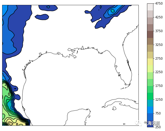
4、地形绘制
 1file_path = single_wrf_file()
 2wrf_file = Dataset(file_path)
 3terrain = getvar(wrf_file, "ter", timeidx=0)
 4cart_proj = get_cartopy(terrain)
 5lats, lons = latlon_coords(terrain)
 6
 7fig = plt.figure(figsize=(10, 7.5))
 8geo_axes = plt.axes(projection=cart_proj)
 9states = NaturalEarthFeature(category='cultural',
10                             scale='50m',
11                             facecolor='none',
12                             name='admin_1_states_provinces_shp')
13geo_axes.add_feature(states, linewidth=.5)
14geo_axes.coastlines('50m', linewidth=0.8)
15levels = numpy.arange(250., 5000., 250.)
16plt.contour(to_np(lons), to_np(lats),
17               to_np(terrain), levels=levels,
18               colors="black",
19               transform=crs.PlateCarree())
20plt.contourf(to_np(lons), to_np(lats),
21                to_np(terrain), levels=levels,
22                transform=crs.PlateCarree(),
23                cmap=get_cmap("terrain"))
24plt.colorbar(ax=geo_axes, shrink=.99)
25plt.show()
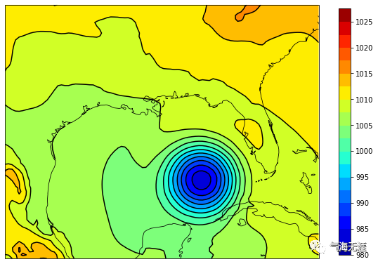
5、海平面气压绘制
 1file_path = single_wrf_file()
 2wrf_file = Dataset(file_path)
 3slp = getvar(wrf_file, "slp", timeidx=0)
 4cart_proj = get_cartopy(slp)
 5lats, lons = latlon_coords(slp)
 6fig = plt.figure(figsize=(10, 7.5))
 7geo_axes = plt.axes(projection=cart_proj)
 8states = NaturalEarthFeature(category='cultural',
 9                             scale='50m',
10                             facecolor='none',
11                             name='admin_1_states_provinces_shp')
12geo_axes.add_feature(states, linewidth=.5)
13geo_axes.coastlines('50m', linewidth=0.8)
14levels = numpy.arange(980.,1030.,2.5)
15plt.contour(to_np(lons), to_np(lats),
16            to_np(slp), levels=levels, colors="black",
17            transform=crs.PlateCarree())
18plt.contourf(to_np(lons), to_np(lats),
19            to_np(slp), levels=levels,
20            transform=crs.PlateCarree(),
21            cmap=get_cmap("jet"))
22plt.colorbar(ax=geo_axes, shrink=.86)
23plt.show()
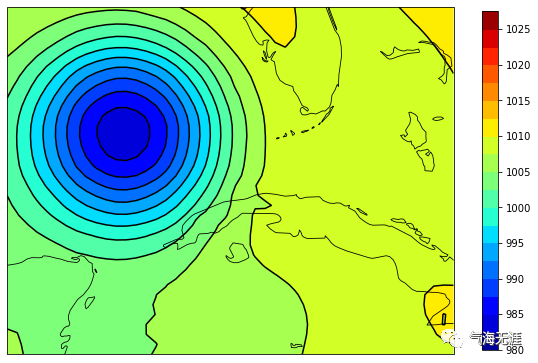
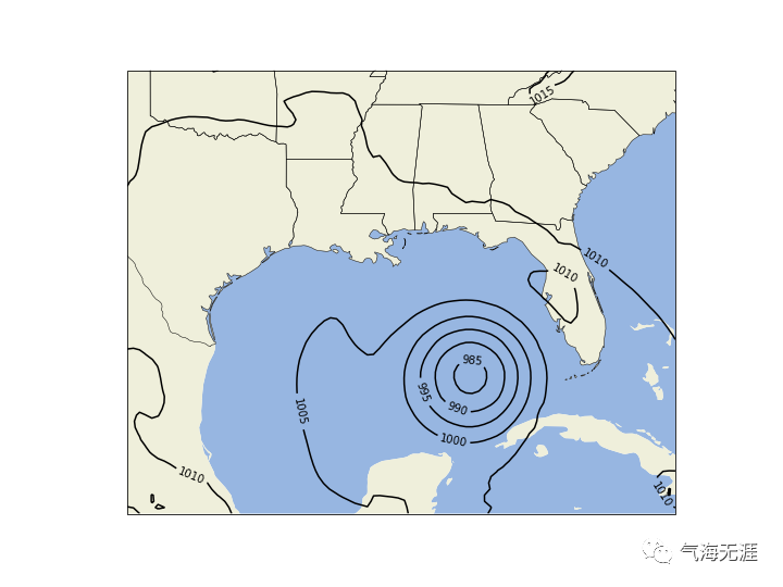
6、截取特定区域绘制海平面气压
 1file_path = single_wrf_file()
 2wrf_file = Dataset(file_path)
 3slp = getvar(wrf_file, "slp", timeidx=0)
 4slp_shape = slp.shape
 5center_y = int(slp_shape[-2]/2.) - 1
 6center_x = int(slp_shape[-1]/2.) - 1
 7
 8slp_quad = slp[..., 0:center_y+1, center_x:]
 9cart_proj = get_cartopy(slp_quad)
10lats, lons = latlon_coords(slp_quad)
11
12fig = plt.figure(figsize=(10, 7.5))
13geo_axes = plt.axes(projection=cart_proj)
14states = NaturalEarthFeature(category='cultural',
15                             scale='50m',
16                             facecolor='none',
17                             name='admin_1_states_provinces_shp')
18geo_axes.add_feature(states, linewidth=.5)
19geo_axes.coastlines('50m', linewidth=0.8)
20levels = numpy.arange(980.,1030.,2.5)
21plt.contour(to_np(lons), to_np(lats),
22            to_np(slp_quad), levels=levels, colors="black",
23            transform=crs.PlateCarree())
24plt.contourf(to_np(lons), to_np(lats),
25            to_np(slp_quad), levels=levels,
26            transform=crs.PlateCarree(),
27            cmap=get_cmap("jet"))
28plt.colorbar(ax=geo_axes, shrink=.83)
29plt.show()
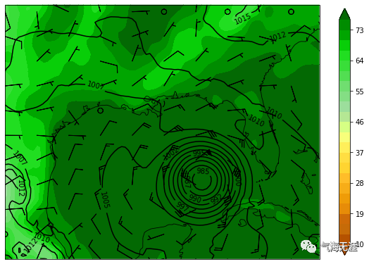
7、气压场和相对湿度绘制
 1file_path = single_wrf_file()
 2wrf_file = Dataset(file_path)
 3
 4slp = getvar(wrf_file, "slp", timeidx=0)
 5td2 = getvar(wrf_file, "td2", timeidx=0, units="degF")
 6u_sfc = getvar(wrf_file, "ua", timeidx=0, units="kt")[0,:]
 7v_sfc = getvar(wrf_file, "va", timeidx=0, units="kt")[0,:]
 8
 9cart_proj = get_cartopy(slp)
10lats, lons = latlon_coords(slp)
11
12fig = plt.figure(figsize=(10, 7.5))
13geo_axes = plt.axes(projection=cart_proj)
14
15states = NaturalEarthFeature(category='cultural',
16                             scale='50m',
17                             facecolor='none',
18                             name='admin_1_states_provinces_shp')
19geo_axes.add_feature(states, linewidth=.5)
20geo_axes.coastlines('50m', linewidth=0.8)
21
22slp_levels = numpy.arange(980.,1030.,2.5)
23td2_levels = numpy.arange(10., 79., 3.)
24
25td2_rgb = numpy.array([[181,82,0], [181,82,0],
26                       [198,107,8], [206,107,8],
27                       [231,140,8], [239,156,8],
28                       [247,173,24], [255,189,41],
29                       [255,212,49], [255,222,66],
30                       [255,239,90], [247,255,123],
31                       [214,255,132], [181,231,148],
32                       [156,222,156], [132,222,132],
33                       [112,222,112], [82,222,82],
34                       [57,222,57], [33,222,33],
35                       [8,206,8], [0,165,0],
36                       [0,140,0], [3,105,3]]) / 255.0
37
38td2_cmap, td2_norm = from_levels_and_colors(td2_levels, td2_rgb, extend="both")
39
40slp_contours = plt.contour(to_np(lons),
41                              to_np(lats),
42                              to_np(slp),
43                              levels=slp_levels,
44                              colors="black",
45                              transform=crs.PlateCarree())
46
47plt.contourf(to_np(lons), to_np(lats),
48                to_np(td2), levels=td2_levels,
49                cmap=td2_cmap, norm=td2_norm,
50                extend="both",
51                transform=crs.PlateCarree())
52
53thin = [int(x/10.) for x in lons.shape]
54plt.barbs(to_np(lons[::thin[0], ::thin[1]]),
55             to_np(lats[::thin[0], ::thin[1]]),
56             to_np(u_sfc[::thin[0], ::thin[1]]),
57             to_np(v_sfc[::thin[0], ::thin[1]]),
58             transform=crs.PlateCarree())
59
60plt.clabel(slp_contours, fmt="%i")
61plt.colorbar(ax=geo_axes, shrink=.86, extend="both")
62plt.xlim(cartopy_xlim(slp))
63plt.ylim(cartopy_ylim(slp))
64plt.show()
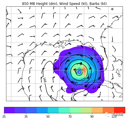
8、850hPa气压场和风场绘制
 1file_path = single_wrf_file()
 2wrf_file = Dataset(file_path)
 3
 4p = getvar(wrf_file, "pressure")
 5z = getvar(wrf_file, "z", units="dm")
 6ua = getvar(wrf_file, "ua", units="kt")
 7va = getvar(wrf_file, "va", units="kt")
 8wspd = getvar(wrf_file, "wspd_wdir", units="kt")[0,:]
 9
10ht_850 = interplevel(z, p, 850)
11u_850 = interplevel(ua, p, 850)
12v_850 = interplevel(va, p, 850)
13wspd_850 = interplevel(wspd, p, 850)
14lats, lons = latlon_coords(ht_850)
15cart_proj = get_cartopy(ht_850)
16
17fig = plt.figure(figsize=(10,7.5))
18ax = plt.axes(projection=cart_proj)
19states = NaturalEarthFeature(category='cultural',
20                             scale='50m',
21                             facecolor='none',
22                             name='admin_1_states_provinces_shp')
23ax.add_feature(states, linewidth=0.5)
24ax.coastlines('50m', linewidth=0.8)
25
26levels = numpy.arange(130., 170., 6.)
27contours = plt.contour(to_np(lons),
28                          to_np(lats),
29                          to_np(ht_850),
30                          levels=levels,
31                          colors="black",
32                          transform=crs.PlateCarree())
33
34plt.clabel(contours, inline=1, fontsize=10, fmt="%i")
35
36levels = [25, 30, 35, 40, 50, 60, 70, 80, 90, 100, 110, 120]
37wspd_contours = plt.contourf(to_np(lons),
38                                to_np(lats),
39                                to_np(wspd_850),
40                                levels=levels,
41                                cmap=get_cmap("rainbow"),
42                                transform=crs.PlateCarree())
43
44plt.colorbar(wspd_contours, ax=ax, orientation="horizontal", pad=.05, shrink=.75)
45
46
47thin = [int(x/10.) for x in lons.shape]
48plt.barbs(to_np(lons[::thin[0], ::thin[1]]),
49          to_np(lats[::thin[0], ::thin[1]]),
50          to_np(u_850[::thin[0], ::thin[1]]),
51          to_np(v_850[::thin[0], ::thin[1]]),
52          length=6,transform=crs.PlateCarree())
53
54# Set the map bounds
55ax.set_xlim(cartopy_xlim(ht_850))
56ax.set_ylim(cartopy_ylim(ht_850))
57
58ax.gridlines()
59
60plt.title("850 MB Height (dm), Wind Speed (kt), Barbs (kt)")
61
62plt.show()
9、垂直剖面绘制
 1cross_start = CoordPair(lat=26.75, lon=-91.7)
 2cross_end = CoordPair(lat=26.75, lon=-86.7)
 3
 4file_path = multiple_wrf_files()
 5wrf_file = [Dataset(x) for x in file_path]
 6
 7
 8slp = getvar(wrf_file, "slp", timeidx=-1)
 9z = getvar(wrf_file, "z", timeidx=-1)
10dbz = getvar(wrf_file, "dbz", timeidx=-1)
11Z = 10**(dbz/10.)
12z_cross = vertcross(Z, z, wrfin=wrf_file,
13                    start_point=cross_start,
14                    end_point=cross_end,
15                    latlon=True, meta=True)
16
17dbz_cross = 10.0 * numpy.log10(z_cross)
18
19lats, lons = latlon_coords(slp)
20cart_proj = get_cartopy(slp)
21
22fig = plt.figure(figsize=(15,5))
23ax_slp = fig.add_subplot(1,2,1,projection=cart_proj)
24ax_dbz = fig.add_subplot(1,2,2)
25
26states = NaturalEarthFeature(category='cultural', scale='50m', facecolor='none',
27                             name='admin_1_states_provinces_shp')
28land = NaturalEarthFeature(category='physical', name='land', scale='50m',
29                           facecolor=COLORS['land'])
30ocean = NaturalEarthFeature(category='physical', name='ocean', scale='50m',
31                            facecolor=COLORS['water'])
32
33
34slp_levels = numpy.arange(950.,1030.,5)
35slp_contours = ax_slp.contour(to_np(lons),
36                              to_np(lats),
37                              to_np(slp),
38                              levels=slp_levels,
39                              colors="black",
40                              zorder=3,
41                              transform=crs.PlateCarree())
42
43ax_slp.clabel(slp_contours, fmt="%i")
44
45ax_slp.plot([cross_start.lon, cross_end.lon],
46            [cross_start.lat, cross_end.lat],
47            color="yellow",
48            marker="o",
49            zorder=3,
50            transform=crs.PlateCarree())
51
52
53ax_slp.add_feature(ocean)
54ax_slp.add_feature(land)
55ax_slp.add_feature(states, linewidth=.5, edgecolor="black")
56
57
58dbz_levels = numpy.arange(5.,75.,5.)
59dbz_contours = ax_dbz.contourf(to_np(dbz_cross), levels=dbz_levels, cmap=get_cmap("jet"))
60cb_dbz = fig.colorbar(dbz_contours, ax=ax_dbz)
61cb_dbz.ax.tick_params(labelsize=8)
62
63
64coord_pairs = to_np(dbz_cross.coords["xy_loc"])
65x_ticks = numpy.arange(coord_pairs.shape[0])
66x_labels = [pair.latlon_str() for pair in to_np(coord_pairs)]
67
68thin = [int(x/5.) for x in x_ticks.shape]
69ax_dbz.set_xticks(x_ticks[1::thin[0]])
70ax_dbz.set_xticklabels(x_labels[::thin[0]], rotation=45, fontsize=8)
71
72
73vert_vals = to_np(dbz_cross.coords["vertical"])
74v_ticks = numpy.arange(vert_vals.shape[0])
75
76thin = [int(x/8.) for x in v_ticks.shape]
77ax_dbz.set_yticks(v_ticks[::thin[0]])
78ax_dbz.set_yticklabels(vert_vals[::thin[0]], fontsize=8)
79
80ax_dbz.set_xlabel("Latitude, Longitude", fontsize=12)
81ax_dbz.set_ylabel("Height (m)", fontsize=12)
82
83ax_slp.set_title("Sea Level Pressure (hPa)", {"fontsize" : 14})
84ax_dbz.set_title("Cross-Section of Reflectivity (dBZ)", {"fontsize" : 14})
85
86plt.show()

10、时空演变绘制(动画与视频)
 1file_path = multiple_wrf_files()
 2wrf_file = [Dataset(f) for f in file_path]
 3slp_all = getvar(wrf_file, "slp", timeidx=ALL_TIMES)
 4cart_proj = get_cartopy(slp_all)
 5fig = plt.figure(figsize=(10,7.5))
 6ax_slp = plt.axes(projection=cart_proj)
 7states = NaturalEarthFeature(category='cultural', scale='50m', facecolor='none',
 8                                      name='admin_1_states_provinces_shp')
 9land = NaturalEarthFeature(category='physical', name='land', scale='50m',
10                                    facecolor=COLORS['land'])
11ocean = NaturalEarthFeature(category='physical', name='ocean', scale='50m',
12                                     facecolor=COLORS['water'])
13slp_levels = numpy.arange(950.,1030.,5.)
14num_frames = slp_all.shape[0]
15
16def animate(i):
17    ax_slp.clear()
18    slp = slp_all[i,:]
19
20    lats, lons = latlon_coords(slp)
21
22    ax_slp.add_feature(ocean)
23    ax_slp.add_feature(land)
24    ax_slp.add_feature(states, linewidth=.5, edgecolor="black")
25    slp_contours = ax_slp.contour(to_np(lons),
26                                  to_np(lats),
27                                  to_np(slp),
28                                  levels=slp_levels,
29                                  colors="black",
30                                  zorder=5,
31                                  transform=crs.PlateCarree())
32    ax_slp.clabel(slp_contours, fmt="%i")
33    ax_slp.set_xlim(cartopy_xlim(slp))
34    ax_slp.set_ylim(cartopy_ylim(slp))
35    return ax_slp
36
37
38ani = FuncAnimation(fig, animate, num_frames, interval=500)
39HTML(ani.to_jshtml())
注:此处的动画演示请到原文中查看
1HTML(ani.to_html5_video())
有问题可以到QQ群里进行讨论,我们在那边等大家。
QQ群号:854684131
文章转载自气海无涯,如果涉嫌侵权,请发送邮件至:contact@modb.pro进行举报,并提供相关证据,一经查实,墨天轮将立刻删除相关内容。
