Python气象数据处理与绘图：3D 插值

本次数据涉及3个维度：经度，纬度，时间

1、导入模块

 1import cartopy.crs
 2import matplotlib
 3import matplotlib.pyplot
 4import numpy
 5import pyinterp
 6import pyinterp.backends.xarray
 7import xarray
 8
 9import warnings
10warnings.filterwarnings('ignore')

2、读取数据

1ds = xarray.open_dataset("tcw.nc")
2interpolator = pyinterp.backends.xarray.Grid3D(ds.tcw)

3、创建网格

1mx, my, mz = numpy.meshgrid(numpy.arange(-180, 180, 0.25) + 1 / 3.0,
2                            numpy.arange(-80, 80, 0.25) + 1 / 3.0,
3                            numpy.array(["2002-07-02T15:00:00"], dtype="datetime64"),
4                            indexing='ij')

4、选择插值函数（trivariate）

1trivariate = interpolator.trivariate(dict(longitude=mx.flatten(), latitude=my.flatten(), time=mz.flatten()))
2interpolator = pyinterp.backends.xarray.Grid3D(ds.data_vars["tcw"],increasing_axes=True)

5、选择插值函数（bicubic）

1bicubic = interpolator.bicubic(
2    dict(longitude=mx.flatten(), latitude=my.flatten(), time=mz.flatten()))

6、进行数据插值

1trivariate = trivariate.reshape(mx.shape).squeeze(axis=2)
2bicubic = bicubic.reshape(mx.shape).squeeze(axis=2)
3lons = mx[:, 0].squeeze()
4lats = my[0, :].squeeze()

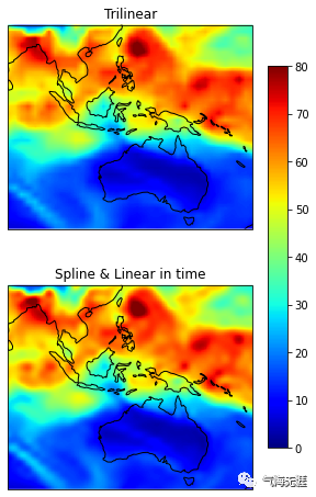
7、可视化插值结果

 1fig = matplotlib.pyplot.figure(figsize=(5, 8))
 2ax1 = fig.add_subplot(
 3    211, projection=cartopy.crs.PlateCarree(central_longitude=180))
 4pcm = ax1.pcolormesh(lons,
 5                     lats,
 6                     trivariate.T,
 7                     cmap='jet',
 8                     transform=cartopy.crs.PlateCarree(),
 9                     vmin=0,
10                     vmax=80)
11ax1.coastlines()
12ax1.set_extent([80, 170, -45, 30], crs=cartopy.crs.PlateCarree())
13ax1.set_title("Trilinear")
14
15ax2 = fig.add_subplot(
16    212, projection=cartopy.crs.PlateCarree(central_longitude=180))
17pcm = ax2.pcolormesh(lons,
18                     lats,
19                     bicubic.T,
20                     cmap='jet',
21                     transform=cartopy.crs.PlateCarree(),
22                     vmin=0,
23                     vmax=80)
24ax2.coastlines()
25ax2.set_extent([80, 170, -45, 30], crs=cartopy.crs.PlateCarree())
26ax2.set_title("Spline & Linear in time")
27fig.colorbar(pcm, ax=[ax1, ax2], shrink=0.8)
28fig.show()