Python气象数据处理与绘图：Cartopy绘制不同投影的地图

1、导入模块

1import numpy as np
2import matplotlib.pyplot as plt
3import cartopy.crs as ccrs
4import cartopy.io.shapereader as shpreader
5import cartopy.feature as cfeat
6import shapely.geometry as sgeom
7import shapefile

2、加载矢量数据

1world = shpreader.Reader('/home/kesci/work/map/world.shp')

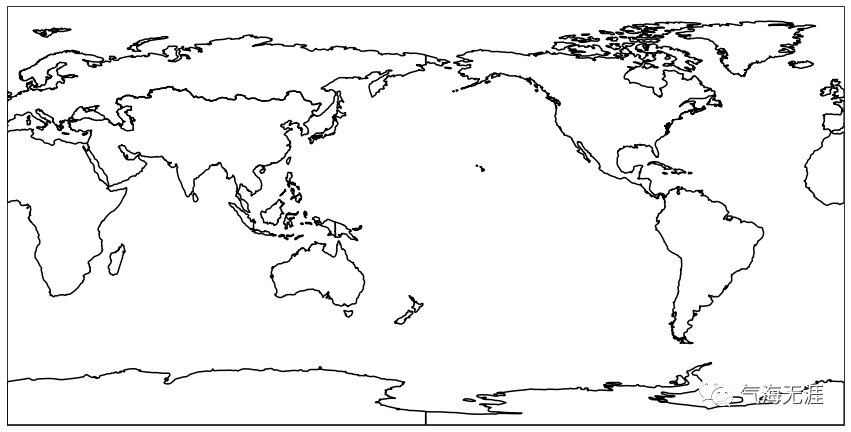
3、绘图

1fig = plt.figure(figsize=(15, 15))
2ax = fig.add_subplot(1, 1, 1, projection=ccrs.PlateCarree())
3ax.set_global()
4ax.add_geometries(world.geometries(), crs=ccrs.PlateCarree(), linewidths=1.5,edgecolor='k',facecolor='none')
5plt.show()

1fig = plt.figure(figsize=(15, 15))
2ax = fig.add_subplot(1, 1, 1, projection=ccrs.AlbersEqualArea(central_longitude=110))
3ax.set_global()
4ax.add_geometries(world.geometries(), crs=ccrs.PlateCarree(), linewidths=1.5,edgecolor='k',facecolor='none')
5plt.show()

1fig = plt.figure(figsize=(15, 15))
2ax = fig.add_subplot(1, 1, 1, projection=ccrs.AzimuthalEquidistant())
3ax.set_global()
4ax.add_geometries(world.geometries(), crs=ccrs.PlateCarree(), linewidths=1.5,edgecolor='k',facecolor='none')
5plt.show()

1fig = plt.figure(figsize=(15, 15))
2ax = fig.add_subplot(1, 1, 1, projection=ccrs.EquidistantConic())
3ax.set_global()
4ax.add_geometries(world.geometries(), crs=ccrs.PlateCarree(), linewidths=1.5,edgecolor='k',facecolor='none')
5plt.show()

1fig = plt.figure(figsize=(15, 15))
2ax = fig.add_subplot(1, 1, 1, projection=ccrs.LambertConformal())
3ax.set_global()
4ax.add_geometries(world.geometries(), crs=ccrs.PlateCarree(), linewidths=1.5,edgecolor='k',facecolor='none')
5plt.show()

1fig = plt.figure(figsize=(15, 15))
2ax = fig.add_subplot(1, 1, 1, projection=ccrs.LambertCylindrical())
3ax.set_global()
4ax.add_geometries(world.geometries(), crs=ccrs.PlateCarree(), linewidths=1.5,edgecolor='k',facecolor='none')
5plt.show()

1fig = plt.figure(figsize=(15, 15))
2ax = fig.add_subplot(1, 1, 1, projection=ccrs.Miller())
3ax.set_global()
4ax.add_geometries(world.geometries(), crs=ccrs.PlateCarree(), linewidths=1.5,edgecolor='k',facecolor='none')
5plt.show()

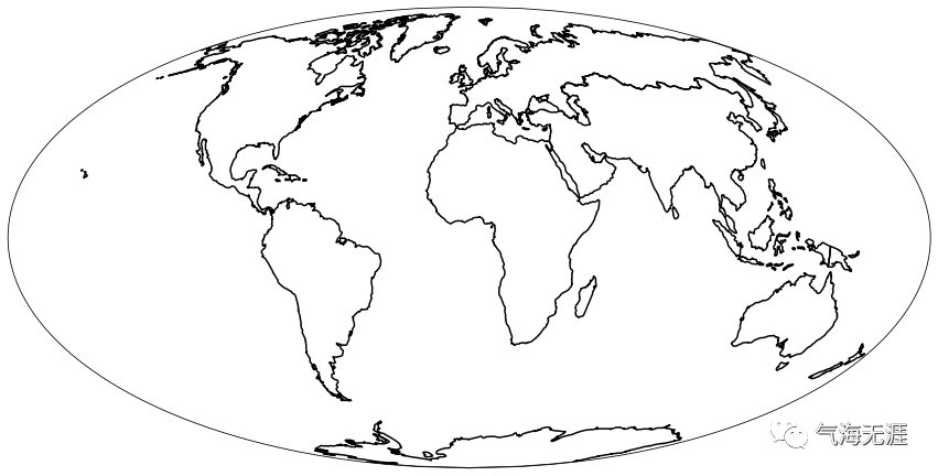
1fig = plt.figure(figsize=(15, 15))
2ax = fig.add_subplot(1, 1, 1, projection=ccrs.Mollweide())
3ax.set_global()
4ax.add_geometries(world.geometries(), crs=ccrs.PlateCarree(), linewidths=1.5,edgecolor='k',facecolor='none')
5plt.show()

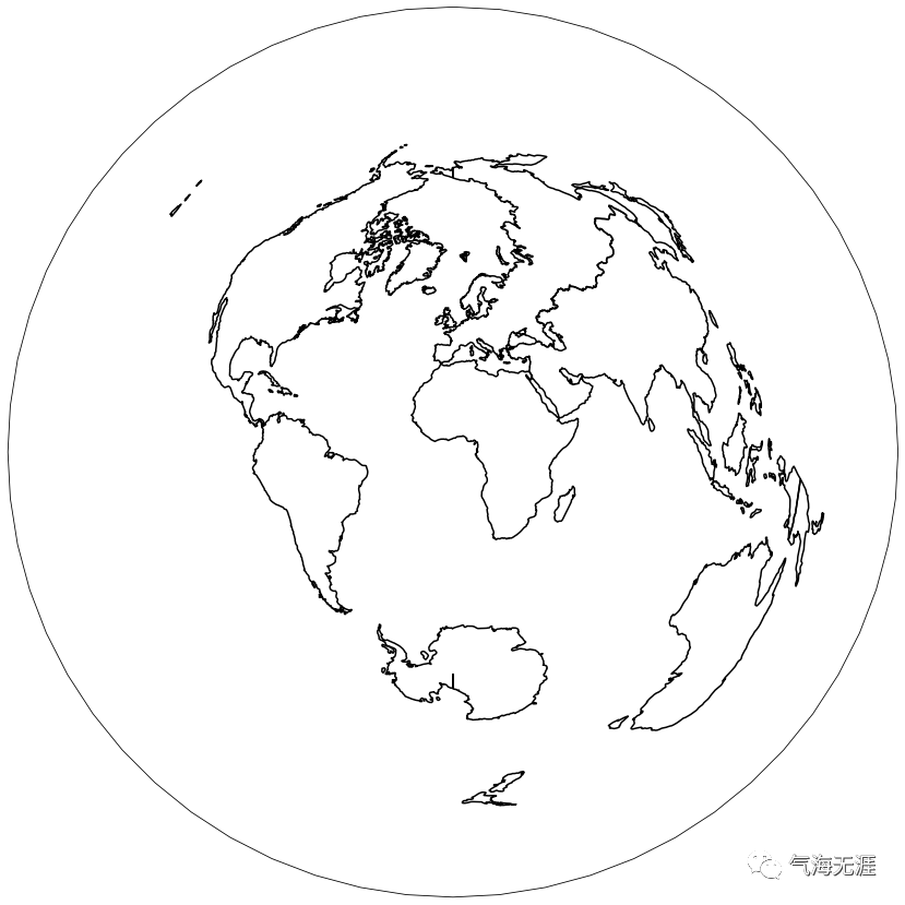
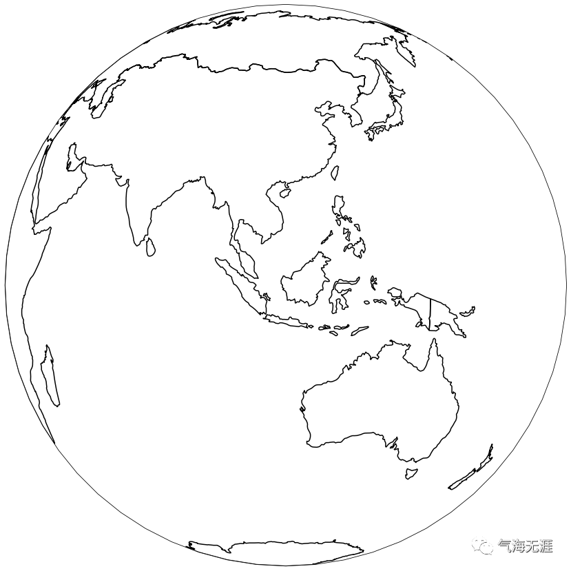
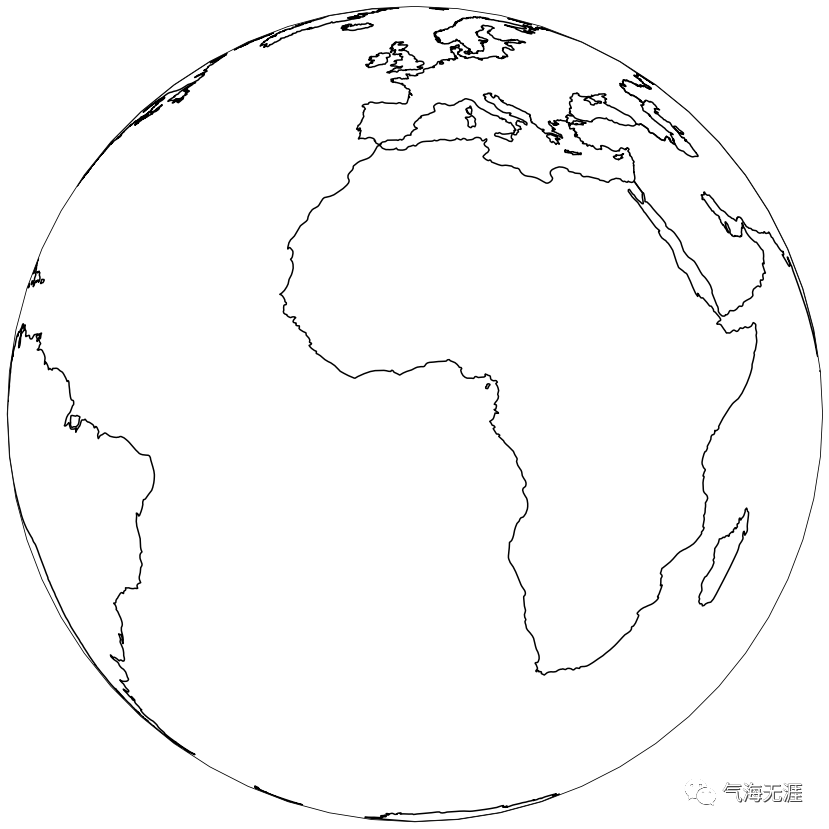
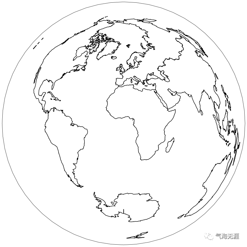
1fig = plt.figure(figsize=(15, 15))
2ax = fig.add_subplot(1, 1, 1, projection=ccrs.Orthographic(central_longitude=110))
3ax.set_global()
4ax.add_geometries(world.geometries(), crs=ccrs.PlateCarree(), linewidths=1.5,edgecolor='k',facecolor='none')
5plt.show()

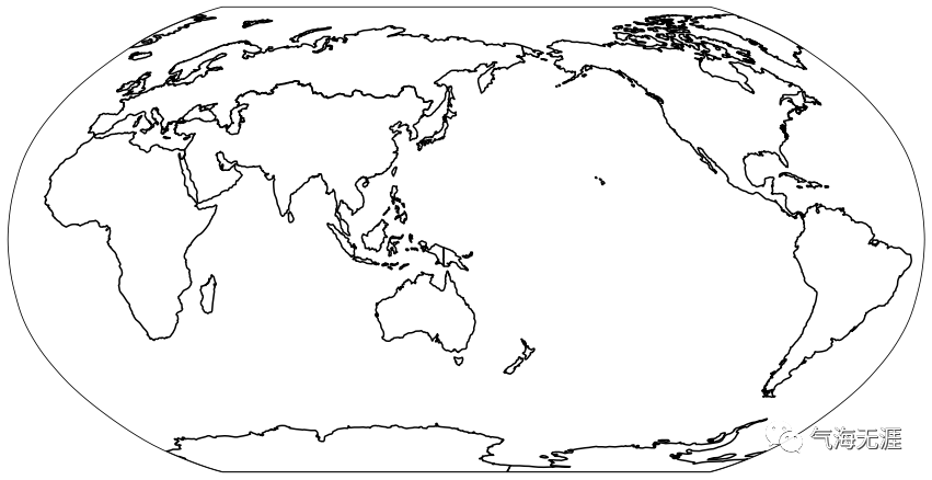
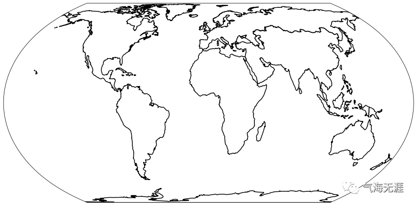
1fig = plt.figure(figsize=(15, 15))
2ax = fig.add_subplot(1, 1, 1, projection=ccrs.Robinson(central_longitude=150))
3ax.set_global()
4ax.add_geometries(world.geometries(), crs=ccrs.PlateCarree(), linewidths=1.5,edgecolor='k',facecolor='none')
5plt.show()

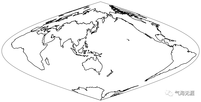
1fig = plt.figure(figsize=(15, 15))
2ax = fig.add_subplot(1, 1, 1, projection=ccrs.Sinusoidal(central_longitude=150))
3ax.set_global()
4ax.add_geometries(world.geometries(), crs=ccrs.PlateCarree(), linewidths=1.5,edgecolor='k',facecolor='none')
5plt.show()

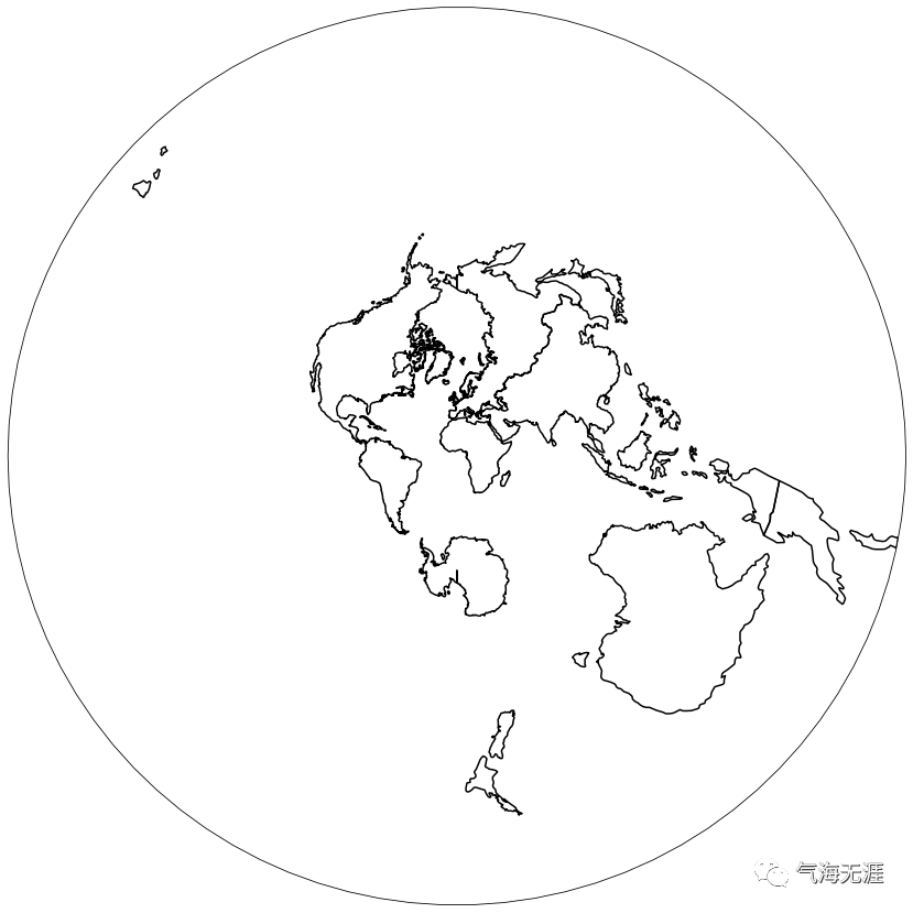
1fig = plt.figure(figsize=(15, 15))
2ax = fig.add_subplot(1, 1, 1, projection=ccrs.Stereographic())
3ax.set_global()
4ax.add_geometries(world.geometries(), crs=ccrs.PlateCarree(), linewidths=1.5,edgecolor='k',facecolor='none')
5plt.show()

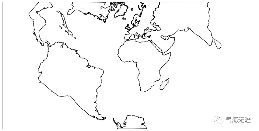
1fig = plt.figure(figsize=(15, 15))
2ax = fig.add_subplot(1, 1, 1, projection=ccrs.TransverseMercator())
3ax.set_global()
4ax.add_geometries(world.geometries(), crs=ccrs.PlateCarree(), linewidths=1.5,edgecolor='k',facecolor='none')
5plt.show()

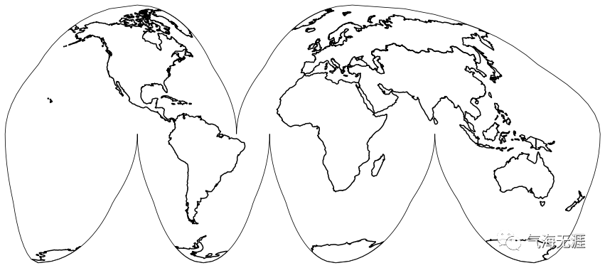
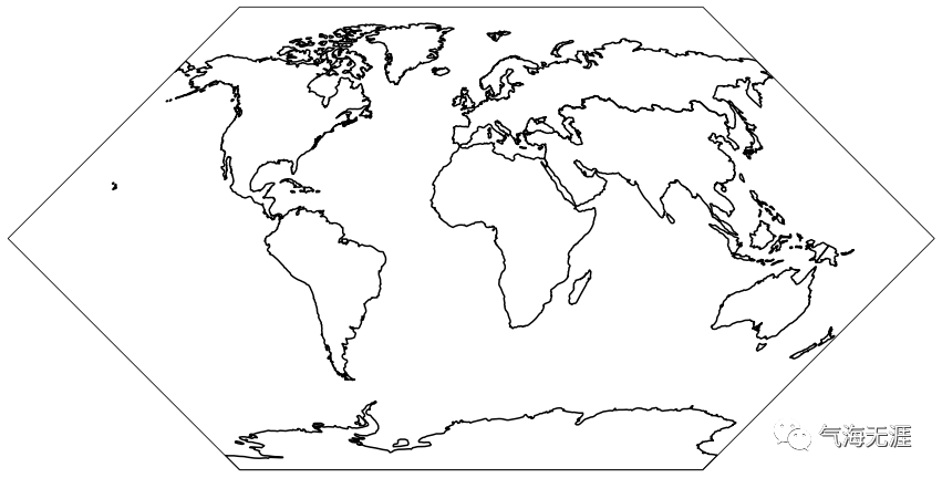
1fig = plt.figure(figsize=(15, 15))
2ax = fig.add_subplot(1, 1, 1, projection=ccrs.InterruptedGoodeHomolosine())
3ax.set_global()
4ax.add_geometries(world.geometries(), crs=ccrs.PlateCarree(), linewidths=1.5,edgecolor='k',facecolor='none')
5plt.show()

1fig = plt.figure(figsize=(15, 15))
2ax = fig.add_subplot(1, 1, 1, projection=ccrs.RotatedPole())
3ax.set_global()
4ax.add_geometries(world.geometries(), crs=ccrs.PlateCarree(), linewidths=1.5,edgecolor='k',facecolor='none')
5plt.show()

1fig = plt.figure(figsize=(15, 15))
2ax = fig.add_subplot(1, 1, 1, projection=ccrs.Geostationary())
3ax.set_global()
4ax.add_geometries(world.geometries(), crs=ccrs.PlateCarree(), linewidths=1.5,edgecolor='k',facecolor='none')
5plt.show()

1fig = plt.figure(figsize=(15, 15))
2ax = fig.add_subplot(1, 1, 1, projection=ccrs.EckertI())
3ax.set_global()
4ax.add_geometries(world.geometries(), crs=ccrs.PlateCarree(), linewidths=1.5,edgecolor='k',facecolor='none')
5plt.show()

1fig = plt.figure(figsize=(15, 15))
2ax = fig.add_subplot(1, 1, 1, projection=ccrs.EqualEarth())
3ax.set_global()
4ax.add_geometries(world.geometries(), crs=ccrs.PlateCarree(), linewidths=1.5,edgecolor='k',facecolor='none')
5plt.show()

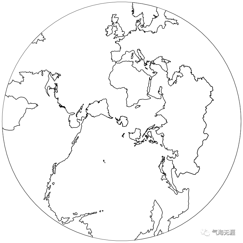
1fig = plt.figure(figsize=(15, 15))
2ax = fig.add_subplot(1, 1, 1, projection=ccrs.LambertAzimuthalEqualArea())
3ax.set_global()
4ax.add_geometries(world.geometries(), crs=ccrs.PlateCarree(), linewidths=1.5,edgecolor='k',facecolor='none')
5plt.show()

1fig = plt.figure(figsize=(15, 15))
2ax = fig.add_subplot(1, 1, 1, projection=ccrs.SouthPolarStereo())
3ax.set_global()
4ax.add_geometries(world.geometries(), crs=ccrs.PlateCarree(), linewidths=1.5,edgecolor='k',facecolor='none')
5plt.show()