Python气象数据处理与绘图：我国地形(DEM)数据可视化

一、导入模块

1%matplotlib inline
2import numpy as np
3import matplotlib.pyplot as plt
4import gdal
5import cmaps

二、读取数据（方法一）

1ds = gdal.Open('/home/kesci/input/DEM2203/dem_1km.tif')
2dem = ds.ReadAsArray()
3dem

1array([[-32768, -32768, -32768, ..., -32768, -32768, -32768],
2       [-32768, -32768, -32768, ..., -32768, -32768, -32768],
3       [-32768, -32768, -32768, ..., -32768, -32768, -32768],
4       ...,
5       [-32768, -32768, -32768, ..., -32768, -32768, -32768],
6       [-32768, -32768, -32768, ..., -32768, -32768, -32768],
7       [-32768, -32768, -32768, ..., -32768, -32768, -32768]], dtype=int16)

检查行数和列数

1nrows  =  ds.RasterXSize  
2ncols  =  ds.RasterYSize
3print('行数；{}\n列数：{}'.format(nrows,ncols))

输出：

1行数；8882
2列数：5043

三、读取数据（方法二）

1band = ds.GetRasterBand(1) 
2dem = band.ReadAsArray(0, 0,nrows, ncols)
3dem

输出：

1array([[-32768, -32768, -32768, ..., -32768, -32768, -32768],
2       [-32768, -32768, -32768, ..., -32768, -32768, -32768],
3       [-32768, -32768, -32768, ..., -32768, -32768, -32768],
4       ...,
5       [-32768, -32768, -32768, ..., -32768, -32768, -32768],
6       [-32768, -32768, -32768, ..., -32768, -32768, -32768],
7       [-32768, -32768, -32768, ..., -32768, -32768, -32768]], dtype=int16)

打印dem shape

1dem.shape

输出：

1(5043, 8882)

四、缺失值掩膜

掩膜代码：

1masked_dem = np.ma.masked_equal(dem, -32768)
2masked_dem

输出：

 1masked_array(
 2  data=[[--, --, --, ..., --, --, --],
 3        [--, --, --, ..., --, --, --],
 4        [--, --, --, ..., --, --, --],
 5        ...,
 6        [--, --, --, ..., --, --, --],
 7        [--, --, --, ..., --, --, --],
 8        [--, --, --, ..., --, --, --]],
 9  mask=[[ True,  True,  True, ...,  True,  True,  True],
10        [ True,  True,  True, ...,  True,  True,  True],
11        [ True,  True,  True, ...,  True,  True,  True],
12        ...,
13        [ True,  True,  True, ...,  True,  True,  True],
14        [ True,  True,  True, ...,  True,  True,  True],
15        [ True,  True,  True, ...,  True,  True,  True]],
16  fill_value=-32768,
17  dtype=int16)

五、绘制快视图

1fig, ([ax1, ax2, ax3]) = plt.subplots(1, 3, figsize=(18, 6))
2ax1.imshow(masked_dem,cmap = plt.cm.gray)
3ax1.set_axis_off()
4ax2.imshow(masked_dem,cmap = plt.cm.jet)
5ax2.set_axis_off()
6ax3.imshow(masked_dem,cmap = plt.cm.gist_earth)
7ax3.set_axis_off()

六、查看地理坐标属性

1gt = ds.GetGeoTransform()
2gt

输出：

1(66.39631807062933,
2 0.008062025005123128,
3 0.0,
4 55.56392411034749,
5 0.0,
6 -0.008062025005123128)

1xres = gt[1]
2yres = gt[5]
3xmin = gt[0] + xres * 0.5
4xmax = gt[0] + (xres * ds.RasterXSize) - xres * 0.5
5ymin = gt[3] + (yres * ds.RasterYSize) + yres * 0.5
6ymax = gt[3] - yres * 0.5
7lons, lats = np.mgrid[xmin:xmax+xres:xres, ymax+yres:ymin:yres]

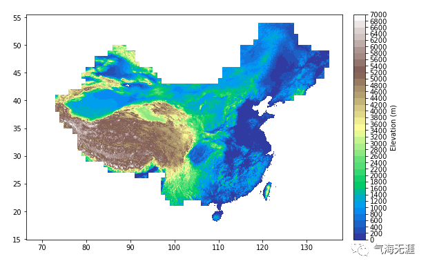
七、绘制地形渲染图

绘图代码1：

1plt.figure(figsize=(10,6))
2levels = np.linspace(0,7000,36)
3ticks = np.linspace(0,7000,36)
4cs = plt.contourf(lons, lats, masked_dem.T, levels=levels, cmap=cmaps.MPL_terrain)
5plt.colorbar(cs, pad=0.03, ticks=ticks, label='Elevation (m)')
6plt.show()

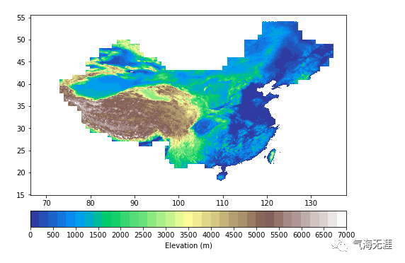
绘图代码2：

1plt.figure(figsize=(8,6))
2levels = np.linspace(0,7000,36)
3ticks = np.linspace(0,7000,15)
4cs = plt.contourf(lons, lats, masked_dem.T, levels=levels, cmap=cmaps.MPL_terrain)
5plt.colorbar(cs, orientation='horizontal', pad=0.07, ticks=ticks, label='Elevation (m)')
6plt.show()