


1、前言
之前在简书有发布过Python气象数据处理与绘图(12):轨迹(台风路径,寒潮路径,水汽轨迹)绘制,提问的人比较多,这里我给出比较完整的方法和代码。实际上本质还是循环(应该还有更简便的办法,有思路的小伙伴可以留言反馈)。由于之前的文件过于复杂,这次我重新使用Hysplit模式追踪了一些路径,数据文件供大家测试使用。
2、数据处理
数据文件结构如下:
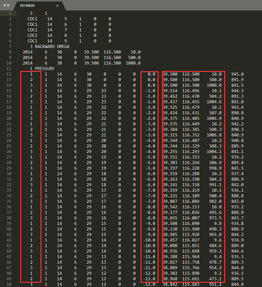
这里解释一下红色框住的部分,(Hysplit模式运行一次默认从10,500,1000米三个高度追踪三条轨迹)第一个框为三条轨迹的序号,第二个框为追踪事件,这里-1.0指的是后向模拟1小时,我文件提供的是后向5天的追踪,所以最后会到-120。第三个框就是三维位置了。我一共提供了5次模拟的数据,一共是5*3=15条轨迹,每个轨迹为121(120+1起点)个时间点。
读取文件:
 1import numpy as np
 2import pandas as pd
 3#建立空数组存放三维位置
 4x = np.zeros((5,3,121),"float")
 5y = np.zeros((5,3,121),"float")
 6z = np.zeros((5,3,121),"float")
 7#读取文件
 8for i in range(5):
 9    f_tmp = pd.read_csv("./{}".format(i),sep='\s+',skiprows=11,header=None, names=['a','b','c','d','e','f','g','h','i','j','k','l','m'])
10    f_tmp = np.array(f_tmp).reshape((121,3, 13))
11    x[i,0,:] = f_tmp[:,0,10]
12    y[i,0,:] = f_tmp[:,0,9]
13    z[i,0,:] = f_tmp[:,0,11]
14    x[i,1,:] = f_tmp[:,1,10]
15    y[i,1,:] = f_tmp[:,1,9]
16    z[i,1,:] = f_tmp[:,1,11]
17    x[i,2,:] = f_tmp[:,2,10]
18    y[i,2,:] = f_tmp[:,2,9]
19    z[i,2,:] = f_tmp[:,2,11]
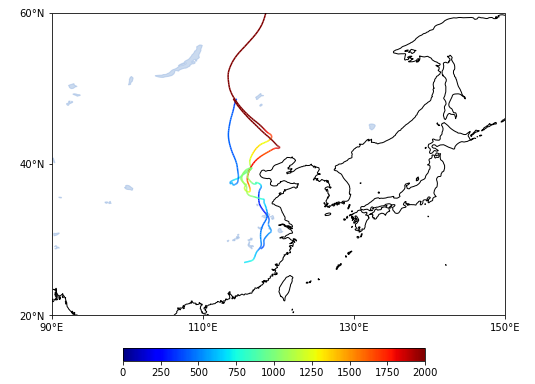
绘制图形(这里只画了5条序号为2的轨迹):
 1from matplotlib.collections import LineCollection
 2import cartopy.crs as ccrs
 3import cartopy.feature as cfeature
 4import matplotlib.pyplot as plt
 5import cartopy.mpl.ticker as cticker
 6#地图底图
 7fig = plt.figure(figsize=(12,7))
 8proj = ccrs.PlateCarree(central_longitude=95)
 9leftlon, rightlon, lowerlat, upperlat = (90,150,20,60)
10img_extent = [leftlon, rightlon, lowerlat, upperlat]
11f_ax1 = fig.add_axes([0.1, 0.1, 0.8, 0.6],projection = proj)
12f_ax1.set_extent(img_extent, crs=ccrs.PlateCarree())
13f_ax1.add_feature(cfeature.COASTLINE.with_scale('50m'))
14f_ax1.add_feature(cfeature.LAKES, alpha=0.5)
15f_ax1.set_xticks(np.arange(leftlon,rightlon+20,20), crs=ccrs.PlateCarree())
16f_ax1.set_yticks(np.arange(lowerlat,upperlat+20,20), crs=ccrs.PlateCarree())
17lon_formatter = cticker.LongitudeFormatter()
18lat_formatter = cticker.LatitudeFormatter()
19f_ax1.xaxis.set_major_formatter(lon_formatter)
20f_ax1.yaxis.set_major_formatter(lat_formatter)
21#轨迹
22for i in range(5):
23    lon = x[i,2,:]
24    lat = y[i,2,:]
25    points = np.array([lon, lat]).T.reshape(-1, 1, 2)#整合经纬度
26    segments = np.concatenate([points[:-1], points[1:]], axis=1)
27    norm = plt.Normalize(0, 2000)#按0-2000的高度对色标标准化
28    lc = LineCollection(segments, cmap='jet', norm=norm,transform=ccrs.PlateCarree())
29    lc.set_array(z[i,2,1:])#颜色色组指定为高度,两个点中间为一条线,所以颜色数组应为点数减1,所以是z[i,2,1:]
30    line = f_ax1.add_collection(lc)
31#色标
32position=fig.add_axes([0.32, 0.01, 0.35, 0.025])
33fig.colorbar(line,cax=position,orientation='horizontal',format='%d')
34plt.show()
输出图形如下:
如需下载测试数据文件,请回复“多轨迹”。
有问题的可以到QQ群里进行讨论,我们在那边等大家。
最后,如果文章对您有帮助的话,欢迎大家花几秒时间点一下赞,在看、收藏、并转发给有需要的同学们,谢谢!

文章转载自气海无涯,如果涉嫌侵权,请发送邮件至:contact@modb.pro进行举报,并提供相关证据,一经查实,墨天轮将立刻删除相关内容。
