关于数据质量管理之正态分布验证

数据质量管理中很重要的一个部分就是数据的离散程度，通常而言，连续值性数据录入是遵循正态分布的，从直方图上容易看，但如何自动化验证数据满足正态分布呢，本文尝试了kstest,normaltest，shaprio等方法，最终结论是建议通过normaltest作为正态分布验证标准，p值>0.05，此外也尝试拓展dataframe.describe，并为以后的数据质量收集做好准备。

代码示例

import numpy as np
import pandas as pd
import matplotlib.pyplot as plt
from scipy import stats

# numpy.random.rand(d0, d1, …, dn)的随机样本位于[0, 1)中
# dataset = pd.DataFrame(np.random.rand(500),columns = ['value'])
# numpy.random.randn(d0, d1, …, dn)是从标准正态分布中返回一个或多个样本值。
dataset = pd.DataFrame(np.random.randn(500,2)+10,columns = ['value1','value2'])
print(dataset.head())
#       value1     value2
# 0   9.343089  10.632460
# 1  12.594335   7.722195
# 2   9.364273  10.625419
# 3   7.974014   9.241017
# 4   9.200326  10.263768
print(dataset.describe())
# dataset.describe()缺省只包括计数、均值、方差、最大值、最小值、25%、50%、75%等信息
#                  value1      value2
# count        500.000000  500.000000
# mean          10.009236   10.003829
# std            1.018261    1.005165
# min            7.345624    7.215147
# 25%            9.335039    9.366773
# 50%            9.921288   10.052754
# 75%           10.652195   10.665082
# max           13.409198   13.481374
dtdesc = dataset.describe()
# 可人工追加均值+3西格玛，均值-3西格玛，上四分位+1.5倍的四分位间距，下四分位-1.5倍的四分位间距
dtdesc.loc['mean+3std'] = dtdesc.loc['mean'] + 3 * dtdesc.loc['std']
#计算平均值-3倍标准差
dtdesc.loc['mean-3std'] = dtdesc.loc['mean'] - 3 * dtdesc.loc['std']
#计算上四分位+1.5倍的四分位间距
dtdesc.loc['75%+1.5dist'] = dtdesc.loc['75%'] + 1.5 * (dtdesc.loc['75%'] - dtdesc.loc['25%'])
#计算下四分位-1.5倍的四分位间距
dtdesc.loc['25%-1.5dist'] = dtdesc.loc['25%'] - 1.5 * (dtdesc.loc['75%'] - dtdesc.loc['25%'])
#                  value1      value2
# mean+3std     13.064018   13.019324
# mean-3std      6.954454    6.988333
# 75%+1.5dist   12.627930   12.612547
# 25%-1.5dist    7.359305    7.419308

# 可再追加各列是否满足正态分布
normaldistribution=[]
for col in dtdesc.columns:
    x = dataset[col]
    u = dataset[col].mean()  # 计算均值
    std = dataset[col].std()  # 计算标准差
    statistic,pvalue = stats.kstest(x, 'norm', (u, std))
    normaldistribution.append(True if pvalue>0.05 else False)
dtdesc.loc['normaldistribution']=normaldistribution
#                       value1    value2
# normaldistribution      True      True

# 构建正态分布数据
# 参数loc(float)：正态分布的均值，对应着这个分布的中心。loc=0说明这一个以Y轴为对称轴的正态分布，
# 参数scale(float)：正态分布的标准差，对应分布的宽度，scale越大，正态分布的曲线越矮胖，scale越小，曲线越高瘦。
# 参数size(int 或者整数元组)：输出的值赋在shape里，默认为None
x = np.random.normal(0,0.963586,500)+9.910642
test_stat = stats.normaltest(x)
# NormaltestResult(statistic=0.008816546859359073, pvalue=0.995601428745786)
x = np.random.normal(0,0.963586,500)
test_stat = stats.normaltest(x)
# NormaltestResult(statistic=0.18462531546355884, pvalue=0.9118200173945978)
x = np.random.normal(0,1,500)
test_stat = stats.normaltest(x)
# NormaltestResult(statistic=1.3984337844262325, pvalue=0.4969743359168226)

# 构建平均值为9.990269，标准差为0.987808，参见上面dataset
x = stats.norm.rvs(loc=9.990269, scale=0.987808, size=(500,))
test_stat = stats.normaltest(x)
# NormaltestResult(statistic=0.6771164970693714, pvalue=0.7127972587837901)

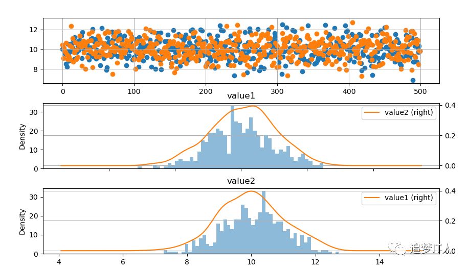
# 创建原始数据图
fig = plt.figure(figsize = (10,6))
ax1 = fig.add_subplot(3,1,1)  # 创建子图,value1和value2的散点图
ax1.scatter(dataset.index, dataset['value1'])
ax1.scatter(dataset.index, dataset['value2'])
plt.grid()
# 绘制数据分布图
ax2 = fig.add_subplot(3,1,2)  # 创建子图,value1的直方图
dataset.hist('value1',bins=50,alpha = 0.5,ax = ax2)
dataset.plot('value1',kind = 'kde', secondary_y=True,ax = ax2)
plt.grid()
ax3 = fig.add_subplot(3,1,3)  # 创建子图,value2的直方图
dataset.hist('value2',bins=50,alpha = 0.5,ax = ax3)
dataset.plot('value2',kind = 'kde', secondary_y=True,ax = ax3)
plt.grid()
plt.show()

def retpddesc(dataset):
    dtdesc = dataset.describe()
    dtdesc.loc['mean+3std'] = dtdesc.loc['mean'] + 3 * dtdesc.loc['std']
    dtdesc.loc['mean-3std'] = dtdesc.loc['mean'] - 3 * dtdesc.loc['std']
    dtdesc.loc['75%+1.5dist'] = dtdesc.loc['75%'] + 1.5 * (dtdesc.loc['75%'] - dtdesc.loc['25%'])
    dtdesc.loc['25%-1.5dist'] = dtdesc.loc['25%'] - 1.5 * (dtdesc.loc['75%'] - dtdesc.loc['25%'])
    kstestvalues=[]
    kstestustdvalues=[]
    normaltestvalues=[]
    shapirovalues=[]
    kstestvaluesflag = []
    kstestustdvaluesflag = []
    normaltestvaluesflag = []
    shapirovaluesflag = []
    for col in dtdesc.columns:
        x = dataset[col]
        statistic, pvalue =stats.normaltest(x)
        kstestvalues.append(pvalue)
        kstestvaluesflag.append(True if pvalue > 0.05 else False)
        statistic, pvalue =stats.kstest(x, 'norm', (u, std))
        kstestustdvalues.append(pvalue)
        kstestustdvaluesflag.append(True if pvalue > 0.05 else False)
        statistic, pvalue =stats.normaltest(x)
        normaltestvalues.append(pvalue)
        normaltestvaluesflag.append(True if pvalue > 0.05 else False)
        statistic, pvalue =stats.shapiro(x)
        shapirovalues.append(pvalue)
        shapirovaluesflag.append(True if pvalue > 0.05 else False)
    dtdesc.loc['kstestvalues'] = kstestvalues
    dtdesc.loc['kstestustdvalues'] = kstestustdvalues
    dtdesc.loc['normaltestvalues'] = normaltestvalues
    dtdesc.loc['shapirovalues'] = shapirovalues
    dtdesc.loc['kstestvaluesflag'] = kstestvaluesflag
    dtdesc.loc['kstestustdvaluesflag'] = kstestustdvaluesflag
    dtdesc.loc['normaltestvaluesflag'] = normaltestvaluesflag
    dtdesc.loc['shapirovaluesflag'] = shapirovaluesflag
    return dtdesc
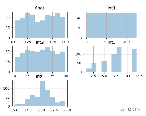
dataset=pd.read_csv("testcsv.csv",header=0)
dataset.describe()
#              int1       float        int2        int3        int4
# count  500.000000  500.000000  500.000000  500.000000  500.000000
# mean   250.500000    0.511262   50.854000    7.700000   20.247487
# std    144.481833    0.286973   27.798168    3.135229    1.949810
# min      1.000000    0.000216    0.000000    1.000000   15.017961
# 25%    125.750000    0.264791   27.000000    5.000000   19.215537
# 50%    250.500000    0.524347   51.000000    8.000000   20.239853
# 75%    375.250000    0.766143   73.000000   12.000000   21.374594
# max    500.000000    0.999791  100.000000   12.000000   24.571841
pddescribe=retpddesc(dataset)
#              int1       float        int2        int3        int4
# 75%+1.5dist           7.495000e+02   1.518171e+00  ...   2.250000e+01   24.613179
# 25%-1.5dist          -2.485000e+02  -4.872369e-01  ...  -5.500000e+00   15.976952
# kstestvalues          1.169302e-69  5.109596e-112  ...   1.614540e-05    0.175321
# kstestustdvalues      0.000000e+00   0.000000e+00  ...  2.580937e-264    0.000000
# normaltestvalues      1.169302e-69  5.109596e-112  ...   1.614540e-05    0.175321
# shapirovalues         2.945411e-11   4.248346e-12  ...   3.732934e-18    0.000060
# kstestvaluesflag      0.000000e+00   0.000000e+00  ...   0.000000e+00    1.000000
# kstestustdvaluesflag  0.000000e+00   0.000000e+00  ...   0.000000e+00    0.000000
# normaltestvaluesflag  0.000000e+00   0.000000e+00  ...   0.000000e+00    1.000000
# shapirovaluesflag     0.000000e+00   0.000000e+00  ...   0.000000e+00    0.000000

dataset.hist(bins=10,alpha = 0.4)
plt.show()

长按二维码关注“追梦IT人”