ARMA-GARCH-COPULA模型和金融时间序列案例

拓端数据部落 2022-07-14

240

原文链接： http://tecdat.cn/?p=3385

最近我被要求撰写关于金融时间序列的copulas的调查。从读取数据中获得各种模型的描述，包括一些图形和统计输出。

相关视频

> oil = read.xlsx（temp，sheetName =“DATA”，dec =“，”）

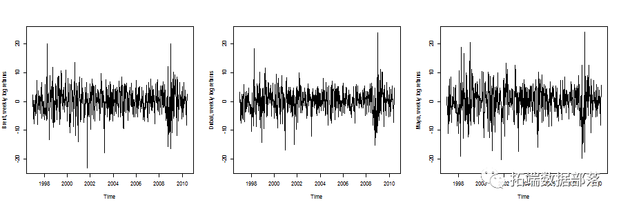
然后我们可以绘制这三个时间序列

1 1997-01-10 2.73672 2.25465 3.3673 1.5400

2 1997-01-17 -3.40326 -6.01433 -3.8249 -4.1076

3 1997-01-24 -4.09531 -1.43076 -6.6375 -4.6166

4 1997-01-31 -0.65789 0.34873 0.7326 -1.5122

5 1997-02-07 -3.14293 -1.97765 -0.7326 -1.8798

6 1997-02-14 -5.60321 -7.84534 -7.6372 -11.0549

这个想法是在这里使用一些多变量ARMA-GARCH过程。这里的启发式是第一部分用于模拟时间序列平均值的动态，第二部分用于模拟时间序列方差的动态。

本文考虑了两种模型

关于ARMA模型残差的多变量GARCH过程（或方差矩阵动力学模型）
关于ARMA-GARCH过程残差的多变量模型（基于copula）

因此，这里将考虑不同的序列，作为不同模型的残差获得。我们还可以将这些残差标准化。

ARMA模型

> fit1 = arima（x = dat \[，1\]，order = c（2,0,1））
> fit2 = arima（x = dat \[，2\]，order = c（1,0,1））
> fit3 = arima（x = dat \[，3\]，order = c（1,0,1））
> m < - apply（dat_arma，2，mean）
> v < - apply（dat_arma，2，var）
> dat\_arma\_std < - t（（t（dat_arma）-m）/ sqrt（v））

ARMA-GARCH模型

> fit1 = garchFit（formula = ~arma（2,1）+ garch（1,1），data = dat \[，1\]，cond.dist =“std”）
> fit2 = garchFit（formula = ~arma（1,1）+ garch（1,1），data = dat \[，2\]，cond.dist =“std”）
> fit3 = garchFit（formula = ~arma（1,1）+ garch（1,1），data = dat \[，3\]，cond.dist =“std”）
> m\_res < - apply（dat\_res，2，mean）
> v\_res < - apply（dat\_res，2，var）
> dat\_res\_std = cbind（（dat\_res \[，1\] -m\_res \[1\]）/ sqrt（v\_res \[1\]），（dat\_res \[，2\] -m\_res \[2\]）/ sqrt（v\_res \[2\]），（dat\_res \[ ，3\] -m\_res \[3\]）/ SQRT（v_res \[3\]））

多变量GARCH模型

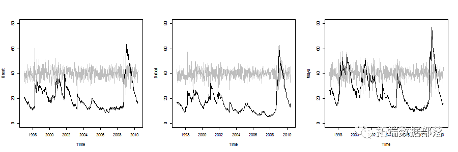
可以考虑的第一个模型是协方差矩阵的多变量EWMA，

> ewma = EWMAvol（dat\_res\_std，lambda = 0.96）

波动性

> emwa\_series\_vol = function（i = 1）{
+ lines（Time，dat_arma \[，i\] + 40，col =“gray”）
+ j = 1
+ if（i == 2）j = 5
+ if（i == 3）j = 9

点击标题查阅往期内容

R语言基于ARMA-GARCH过程的VaR拟合和预测

左右滑动查看更多

隐含相关性

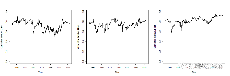
> emwa\_series\_cor = function（i = 1，j = 2）{
+ if（（min（i，j）== 1）＆（max（i，j）== 2））{
+ a = 1; B = 9; AB = 3}
+ r = ewma $ Sigma.t \[，ab\] / sqrt（ewma $ Sigma.t \[，a\] *
+ ewma $ Sigma.t \[，b\]）
+ plot（Time，r，type =“l”，ylim = c（0,1））
+}

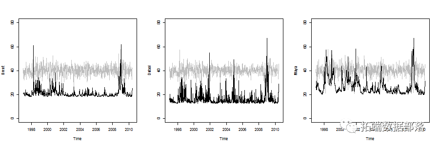
多变量GARCH，即BEKK（1,1）模型，例如使用：

> bekk = BEKK11（dat_arma）
> bekk\_series\_vol function（i = 1）{
+ plot（Time， $ Sigma.t \[，1\]，type =“l”，
+ ylab = （dat）\[i\]，col =“white”，ylim = c（0,80））
+ lines（Time，dat_arma \[，i\] + 40，col =“gray”）
+ j = 1
+ if（i == 2）j = 5

+ if（i == 3）j = 9

> bekk\_series\_cor = function（i = 1，j = 2）{
+ a = 1; B = 5; AB = 2}
+ a = 1; B = 9; AB = 3}
+ a = 5; B = 9; AB = 6}
+ r = bk $ Sigma.t \[，ab\] / sqrt（bk $ Sigma.t \[，a\] *
+ bk $ Sigma.t \[，b\]）

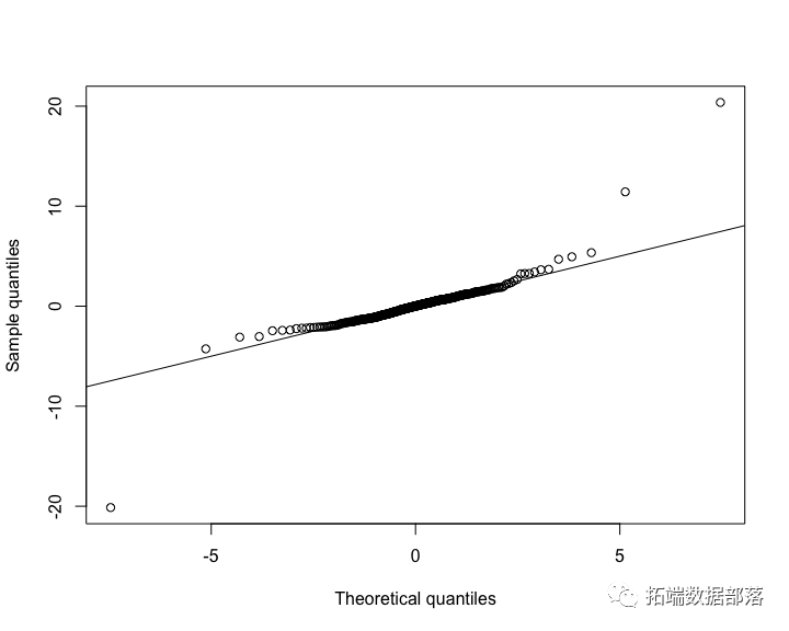
从单变量GARCH模型中模拟残差

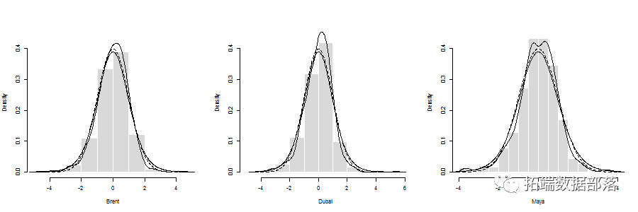
第一步可能是考虑残差的一些静态（联合）分布。单变量边缘分布是

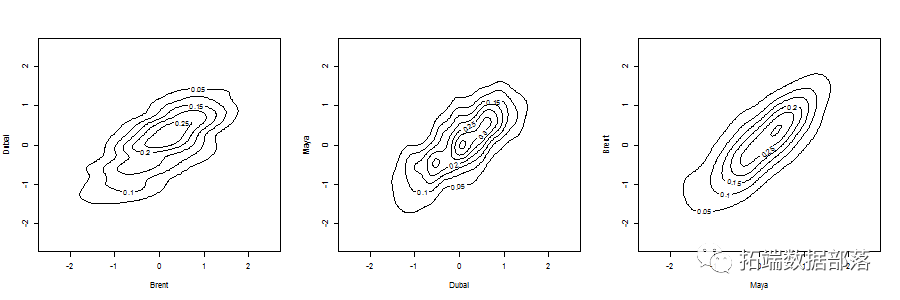
边缘密度的轮廓（使用双变量核估计器获得）

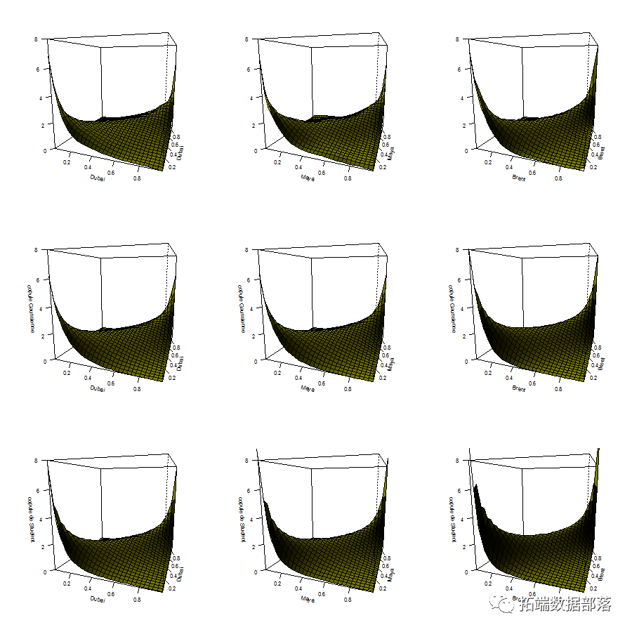
也可以将copula密度可视化（上面有一些非参数估计，下面是参数copula）

> copula_NP = function（i = 1，j = 2）{
+ n = nrow（uv）
+ s = 0.3

+ norm.cop < - normalCopula（0.5）
+ norm.cop < - normalCopula（fitCopula（norm.cop，uv）@estimate）
+ dc = function（x，y）dCopula（cbind（x，y），norm.cop）


+ ylab = names（dat）\[j\]，zlab =“copule Gaussienne”，ticktype =“detailed”，zlim = zl）
+
+ t.cop < - tCopula（0.5，df = 3）
+ t.cop < - tCopula（t.fit \[1\]，df = t.fit \[2\]）


+ ylab = names（dat）\[j\]，zlab =“copule de Student”，ticktype =“detailed”，zlim = zl）
+}

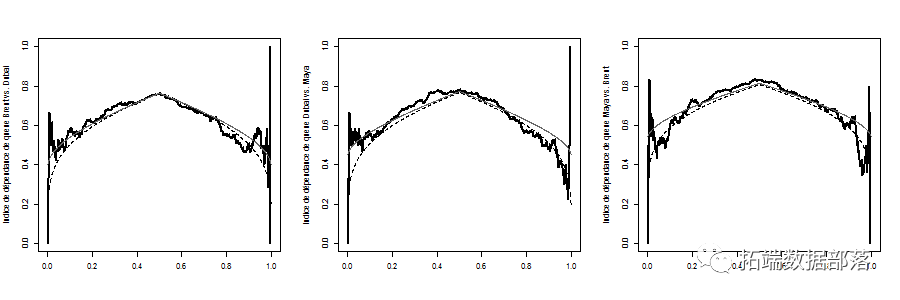
可以考虑这个函数，

计算三个序列的的经验版本，并将其与一些参数版本进行比较，

>

> lambda = function（C）{
+ l = function（u）pcopula（C，cbind（u，u））/ u
+ v = Vectorize（l）（u）
+ return（c（v，rev（v）））
+}
>

> graph_lambda = function（i，j）{
+ X = dat_res
+ U = rank（X \[，i\]）/（nrow（X）+1）
+ V = rank（X \[，j\]）/（nrow（X）+1）

+ normal.cop < - normalCopula（.5，dim = 2）
+ t.cop < - tCopula（.5，dim = 2，df = 3）
+ fit1 = fitCopula（normal.cop，cbind（U，V），method =“ml”）
d（U，V），method =“ml”）
+ C1 = normalCopula（fit1 @ copula @ parameters，dim = 2）
+ C2 = tCopula（fit2 @ copula @ parameters \[1\]，dim = 2，df = trunc（fit2 @ copula @ parameters \[2\]））
+

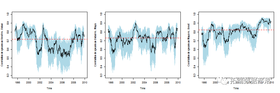
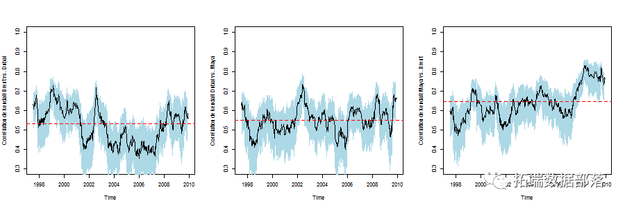
但人们可能想知道相关性是否随时间稳定。

> time\_varying\_correl_2 = function（i = 1，j = 2，
+ nom_arg =“Pearson”）{
+ uv = dat_arma \[，c（i，j）\]
nom_arg））\[1,2\]
+}
> time\_varying\_correl_2（1,2）

> time\_varying\_correl_2（1,2，“spearman”）

> time\_varying\_correl_2（1,2，“kendall”）

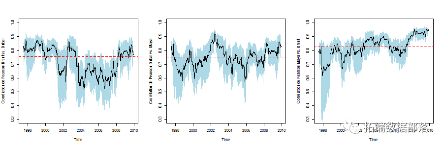
斯皮尔曼与时变排名相关系数

或肯德尔相关系数

为了模型的相关性，考虑DCC模型（S）

> m2 = dccFit（dat\_res\_std）
> m3 = dccFit（dat\_res\_std，type =“Engle”）
> R2 = m2 $ rho.t
> R3 = m3 $ rho.t

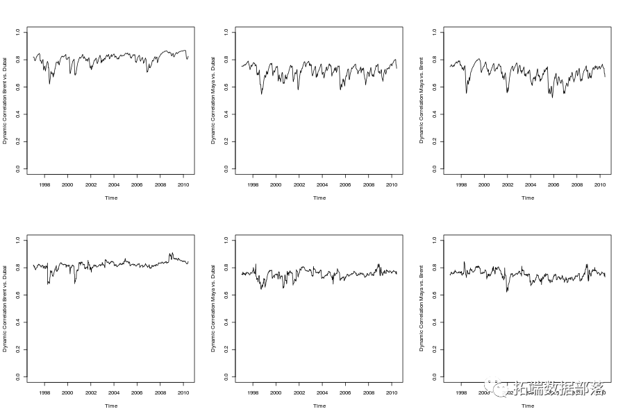
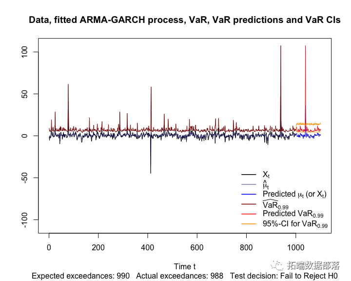
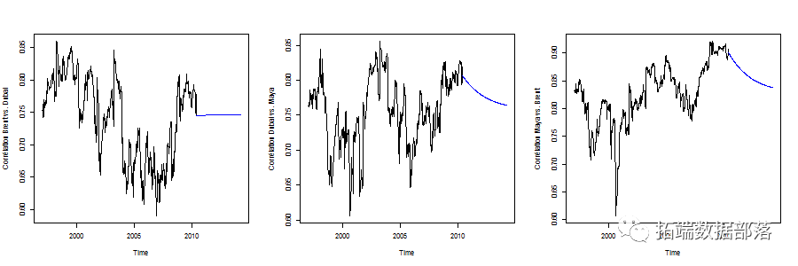
要获得一些预测，使用例如

> garch11.spec = ugarchspec（mean.model = list（armaOrder = c（2,1）），variance.model = list（garchOrder = c（1,1），model =“GARCH”））
> dcc.garch11.spec = dccspec（uspec = multispec（replicate（3，garch11.spec）），dccOrder = c（1,1），
distribution =“mvnorm”）
> dcc.fit = dccfit（dcc.garch11.spec，data = dat）
> fcst = dccforecast（dcc.fit，n.ahead = 200）