


Table of Contents
一. 模型评价指标——Precision/Recall
机器学习(ML),自然语言处理(NLP),信息检索(IR)等领域,评估(Evaluation)是一个必要的 工作,而其评价指标往往有如下几点:准确率(Accuracy),精确率(Precision),召回率(Recall)和F1-Measure。
1.1 准确率、精确率、召回率、F值对比
-
准确率/正确率(Accuracy)= 所有预测正确的样本 / 总的样本 (TP+TN)
-
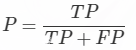
精确率(Precision) = 正类预测为正类(TP) / 所有预测为正类(TP+TN)
-
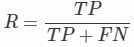
召回率(Recall) = 正类预测为正类(TP) / 所有真正的正类(TP+FN)
-
F值(F-Measure) = 精确率 * 召回率 * 2 / (精确率 + 召回率) —— F值即为精确率和召回率的调和平均值
1.2 精确率、召回率计算公式
1.2.1 精确率计算公式
理解:
-
TP+FP: 也就是全体Positive, 也就是预测的图片中是正类的图片的数目
-
TP: 也就是正类也被预测为正类的图片的个数
总之:预测正确的图片个数占总的正类预测个数的比例(从预测结果角度看,有多少预测是准确的)
1.2.2 召回率计算公式
理解:
-
TP+FN: 也就是全体完全满足图片标注的图片的个数
-
TP:正类被预测为正类的图片个数
总之:确定了正类被预测为正类图片占所有标注图片的个数(从标注角度看,有多少被召回)
1.2.3 F1 score指标
P和R指标有时候会出现的矛盾的情况,这样就需要综合考虑他们,最常见的方法就是F-Measure(又称为F-Score)。
将Precision 和 Recall 结合到一个称为F1 score 的指标,调和平均值给予低值更多权重。因此,如果召回和精确度都很高,分类器将获得高F1分数。
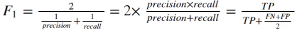
F-Measure是Precision和Recall加权调和平均:
当参数α=1时,就是最常见的F1,也即
可知F1综合了P和R的结果,当F1较高时则能说明试验方法比较有效。
1.3 代码
# 准确率(Precision)和召回率(Recall)
    from sklearn.metrics import precision_score, recall_score

    print(precision_score(y_train_5, y_train_pred))   # 0.7779476399770686
    print(recall_score(y_train_5, y_train_pred))      # 0.7509684560044272

    # F1 score
    from sklearn.metrics import f1_score

    print(f1_score(y_train_5, y_train_pred))          # 0.7642200112633752
二. 模型评估——混淆矩阵(Confusion Matrix)
混淆矩阵是机器学习中总结分类模型预测结果的情形分析表,以矩阵形式将数据集中的记录按照真实的类别与分类模型预测的类别判断两个标准进行汇总。
其中矩阵的行表示真实值,矩阵的列表示预测值。
2.1 案例
已知条件:班级总人数100人,其中男生80人,女生20人。
目标:找出所有的女生。
结果:从班级中选择了50人,其中20人是女生,还错误的把30名男生挑选出来了。
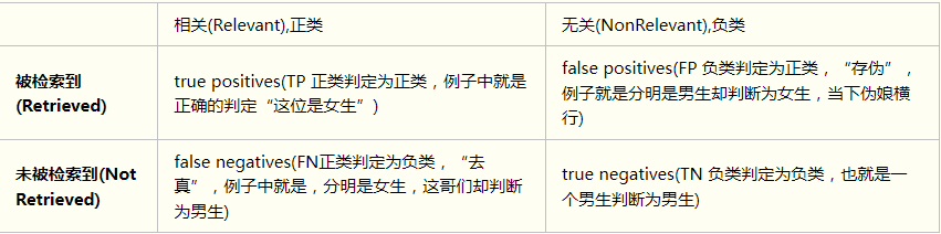
通过这张表,我们可以很容易得到这几个值:TP=20;FP=30;FN=0;TN=50;
-
TP(True Positive):将正类预测为正类数,positive 表示他判定为女生。 true表示,判定是对的。 TP=20
-
FN(False Negative):将正类预测为负类数,negative 表示他判定为男生。 false表示,判定是错的。 FN=0
-
FP(False Positive):将负类预测为正类数, positive 表示他判定为女生。 false表示,判定是错的。 FP=30
-
TN(True Negative):将负类预测为负类数,negative 表示他判定为男生。 true表示, 他的判定是对的。 TN=50
4.2 代码实现
4.2.1 在下采样测试集中计算
代码:
import pandas as pd
import matplotlib.pyplot as plt
import numpy as np
from sklearn.preprocessing import StandardScaler
from sklearn.model_selection import train_test_split
from sklearn.linear_model import LogisticRegression
from sklearn.model_selection import KFold, cross_val_score
from sklearn.metrics import confusion_matrix,recall_score,classification_report
import itertools

def plot_confusion_matrix(cm, classes,
                          title='Confusion matrix',
                          cmap=plt.cm.Blues):
    """
    This function prints and plots the confusion matrix.
    """
    plt.imshow(cm, interpolation='nearest', cmap=cmap)
    plt.title(title)
    plt.colorbar()
    tick_marks = np.arange(len(classes))
    plt.xticks(tick_marks, classes, rotation=0)
    plt.yticks(tick_marks, classes)

    thresh = cm.max() / 2.
    for i, j in itertools.product(range(cm.shape[0]), range(cm.shape[1])):
        plt.text(j, i, cm[i, j],
                 horizontalalignment="center",
                 color="white" if cm[i, j] > thresh else "black")

    plt.tight_layout()
    plt.ylabel('True label')
    plt.xlabel('Predicted label')

data = pd.read_csv("E:/file/creditcard.csv")

# 将金额数据处理成 范围为[-1,1] 之间的数值
# 机器学习默认数值越大,特征就越重要,不处理容易造成的问题是 金额这个特征值的重要性远大于V1-V28特征
data['normAmount'] = StandardScaler().fit_transform(data['Amount'].values.reshape(-1, 1))
# 删除暂时不用的特征值
data = data.drop(['Time','Amount'],axis=1)

X = data.values[:, data.columns != 'Class']
y = data.values[:, data.columns == 'Class']

# 获取异常交易数据的总行数及索引
number_records_fraud = len(data[data.Class == 1])
fraud_indices = np.array(data[data.Class == 1].index)

# 获取正常交易数据的索引值
normal_indices = data[data.Class == 0].index

# 在正常样本当中, 随机采样得到指定个数的样本, 并取其索引
random_normal_indices = np.random.choice(normal_indices, number_records_fraud, replace = False)
random_normal_indices = np.array(random_normal_indices)

# 有了正常和异常的样本后把他们的索引都拿到手
under_sample_indices = np.concatenate([fraud_indices,random_normal_indices])

# 根据索引得到下采样的所有样本点
under_sample_data = data.iloc[under_sample_indices,:]

X_undersample = under_sample_data.loc[:, under_sample_data.columns != 'Class']
y_undersample = under_sample_data.loc[:, under_sample_data.columns == 'Class']

# 对整个数据集进行划分, X为特征数据, Y为标签, test_size为测试集比列, random_state 为随机种子, 目的是使得每次随机的结果都一样
X_train, X_test, y_train, y_test = train_test_split(X, y, test_size=0.3, random_state=0)

# 下采样数据集进行划分
X_train_undersample, X_test_undersample, y_train_undersample, y_test_undersample = train_test_split(X_undersample,y_undersample
                                                                                                   ,test_size = 0.3
                                                                                                   ,random_state = 0)

# 最好的正则惩罚参数 0.01
lr = LogisticRegression(C = 0.01, penalty = 'l2')
lr.fit(X_train_undersample,y_train_undersample.values.ravel())
y_pred_undersample = lr.predict(X_test_undersample.values)

# 计算混淆矩阵
cnf_matrix = confusion_matrix(y_test_undersample,y_pred_undersample)
np.set_printoptions(precision=2)

print("Recall metric in the testing dataset: ", cnf_matrix[1,1]/(cnf_matrix[1,0]+cnf_matrix[1,1]))

# 画出混淆矩阵
class_names = [0,1]
plt.figure()
plot_confusion_matrix(cnf_matrix
                      , classes=class_names
                      , title='Confusion matrix')
plt.show()
测试记录:
Recall metric in the testing dataset: 0.8707482993197279
[外链图片转存失败,源站可能有防盗链机制,建议将图片保存下来直接上传(img-odnnRF57-1658284115120)(https://upload-images.jianshu.io/upload_images/2638478-f96dc45538868a90.png?imageMogr2/auto-orient/strip%7CimageView2/2/w/1240)]
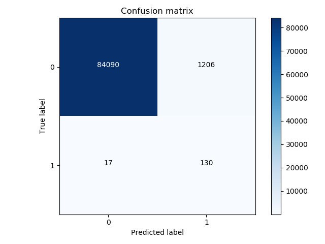
4.2.2 在所有样本的测试集中计算
代码:
# 前面的省略
# 计算混淆矩阵
lr = LogisticRegression(C = 0.01, penalty = 'l2')
lr.fit(X_train_undersample,y_train_undersample.values.ravel())
y_pred = lr.predict(X_test)

# 画出混淆矩阵
cnf_matrix = confusion_matrix(y_test,y_pred)
np.set_printoptions(precision=2)

print("Recall metric in the testing dataset: ", cnf_matrix[1,1]/(cnf_matrix[1,0]+cnf_matrix[1,1]))

# Plot non-normalized confusion matrix
class_names = [0,1]
plt.figure()
plot_confusion_matrix(cnf_matrix
                      , classes=class_names
                      , title='Confusion matrix')
plt.show()
测试记录:
Recall metric in the testing dataset: 0.8843537414965986
参考:
- https://study.163.com/course/introduction.htm?courseId=1003590004#/courseDetail?tab=1
