Table of Contents

• 一. Scikit-Learn阀值概述
• 二. 代码实现
• 参考：

一. Scikit-Learn阀值概述

Scikit-Learn不允许直接设置阈值，但它可以得到决策分数，调用其decision_function()方法，而不是调用分类器的predict()方法，该方法返回每个实例的分数，然后使用想要的阈值根据这些分数进行预测。

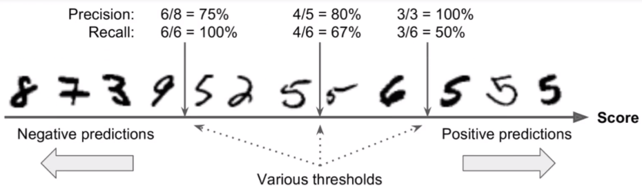
对于这种分类问题，不同的分类阈值可以给出不同的输出结果，但是在sklearn中，无法直接通过直接修改阈值而输出结果，但是我们可以首先得到决策函数得到的结果，然后再手动确定阈值，得到预测的结果。
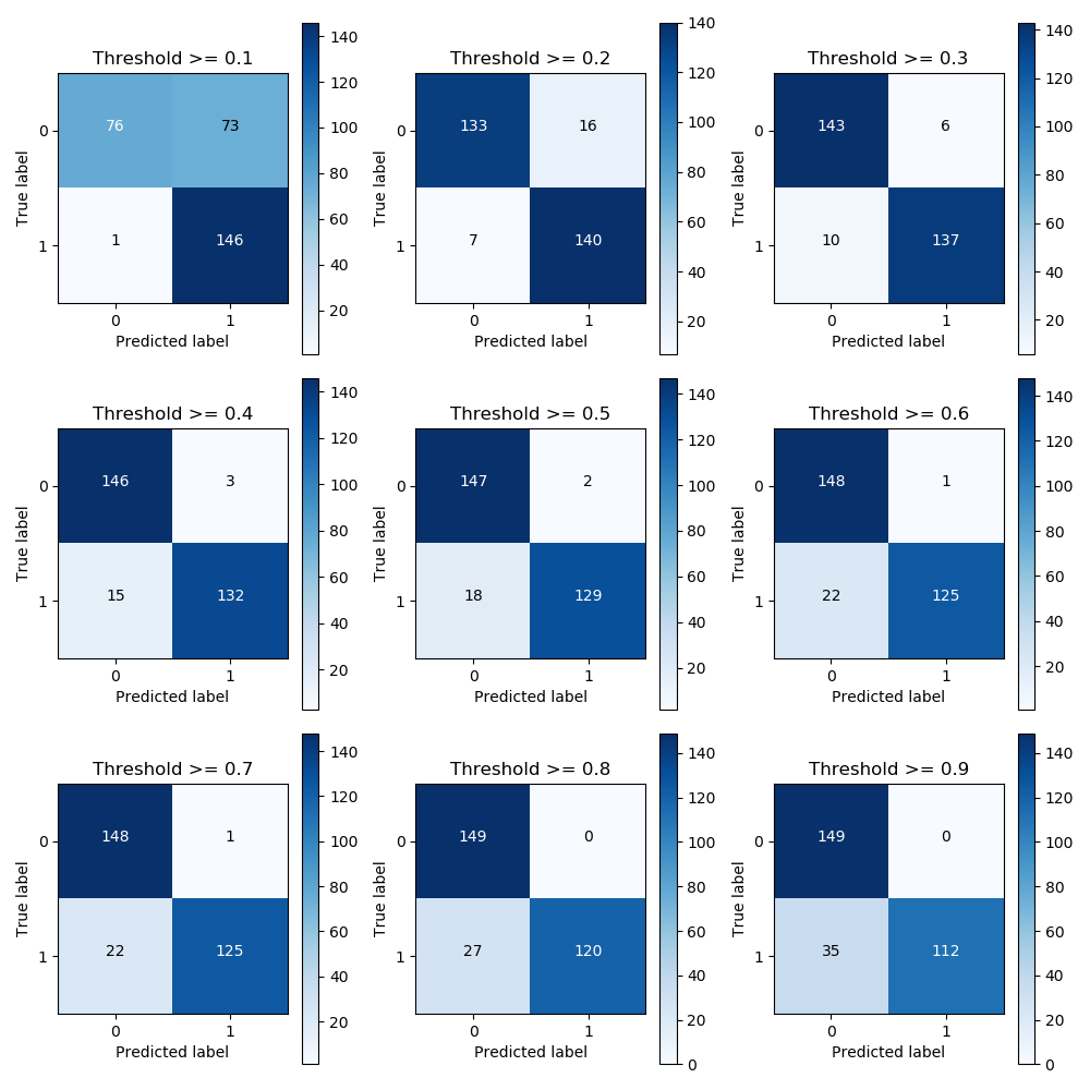
为了使得模型更加完善，我们需要选择合适的阈值，即使得准确率和召回率都比较大，因此在这里我们可以首先绘制出准确率和召回率随阈值的变化关系，然后再选择合适的阈值。

二. 代码实现

代码:

import pandas as pd
import matplotlib.pyplot as plt
import numpy as np
from sklearn.preprocessing import StandardScaler
from sklearn.model_selection import train_test_split
from sklearn.linear_model import LogisticRegression
from sklearn.model_selection import KFold, cross_val_score
from sklearn.metrics import confusion_matrix,recall_score,classification_report
import itertools

def plot_confusion_matrix(cm, classes,
                          title='Confusion matrix',
                          cmap=plt.cm.Blues):
    """
    This function prints and plots the confusion matrix.
    """
    plt.imshow(cm, interpolation='nearest', cmap=cmap)
    plt.title(title)
    plt.colorbar()
    tick_marks = np.arange(len(classes))
    plt.xticks(tick_marks, classes, rotation=0)
    plt.yticks(tick_marks, classes)

    thresh = cm.max() / 2.
    for i, j in itertools.product(range(cm.shape[0]), range(cm.shape[1])):
        plt.text(j, i, cm[i, j],
                 horizontalalignment="center",
                 color="white" if cm[i, j] > thresh else "black")

    plt.tight_layout()
    plt.ylabel('True label')
    plt.xlabel('Predicted label')

data = pd.read_csv("E:/file/creditcard.csv")

# 将金额数据处理成 范围为[-1,1] 之间的数值
# 机器学习默认数值越大，特征就越重要，不处理容易造成的问题是 金额这个特征值的重要性远大于V1-V28特征
data['normAmount'] = StandardScaler().fit_transform(data['Amount'].values.reshape(-1, 1))
# 删除暂时不用的特征值
data = data.drop(['Time','Amount'],axis=1)

X = data.values[:, data.columns != 'Class']
y = data.values[:, data.columns == 'Class']

# 获取异常交易数据的总行数及索引
number_records_fraud = len(data[data.Class == 1])
fraud_indices = np.array(data[data.Class == 1].index)

# 获取正常交易数据的索引值
normal_indices = data[data.Class == 0].index

# 在正常样本当中， 随机采样得到指定个数的样本， 并取其索引
random_normal_indices = np.random.choice(normal_indices, number_records_fraud, replace = False)
random_normal_indices = np.array(random_normal_indices)

# 有了正常和异常的样本后把他们的索引都拿到手
under_sample_indices = np.concatenate([fraud_indices,random_normal_indices])

# 根据索引得到下采样的所有样本点
under_sample_data = data.iloc[under_sample_indices,:]

X_undersample = under_sample_data.loc[:, under_sample_data.columns != 'Class']
y_undersample = under_sample_data.loc[:, under_sample_data.columns == 'Class']

# 对整个数据集进行划分， X为特征数据， Y为标签， test_size为测试集比列， random_state 为随机种子， 目的是使得每次随机的结果都一样
X_train, X_test, y_train, y_test = train_test_split(X, y, test_size=0.3, random_state=0)

# 下采样数据集进行划分
X_train_undersample, X_test_undersample, y_train_undersample, y_test_undersample = train_test_split(X_undersample,y_undersample
                                                                                                   ,test_size = 0.3
                                                                                                   ,random_state = 0)



# 计算混淆矩阵
lr = LogisticRegression(C=0.01, penalty='l2')
lr.fit(X_train_undersample, y_train_undersample.values.ravel())
y_pred_undersample_proba = lr.predict_proba(X_test_undersample.values)

# 指定阀值
thresholds = [0.1, 0.2, 0.3, 0.4, 0.5, 0.6, 0.7, 0.8, 0.9]

plt.figure(figsize=(10, 10))

j = 1
for i in thresholds:
    y_test_predictions_high_recall = y_pred_undersample_proba[:, 1] > i

    plt.subplot(3, 3, j)
    j += 1

    # Compute confusion matrix
    cnf_matrix = confusion_matrix(y_test_undersample, y_test_predictions_high_recall)
    np.set_printoptions(precision=2)

    print("Recall metric in the testing dataset: ", cnf_matrix[1, 1] / (cnf_matrix[1, 0] + cnf_matrix[1, 1]))

    # Plot non-normalized confusion matrix
    class_names = [0, 1]
    plot_confusion_matrix(cnf_matrix
                          , classes=class_names
                          , title='Threshold >= %s' % i)


plt.show()

测试记录:
Recall metric in the testing dataset: 0.9931972789115646
Recall metric in the testing dataset: 0.9523809523809523
Recall metric in the testing dataset: 0.9319727891156463
Recall metric in the testing dataset: 0.8979591836734694
Recall metric in the testing dataset: 0.8775510204081632
Recall metric in the testing dataset: 0.8503401360544217
Recall metric in the testing dataset: 0.8503401360544217
Recall metric in the testing dataset: 0.8163265306122449
Recall metric in the testing dataset: 0.7619047619047619

参考：

1. https://study.163.com/course/introduction.htm?courseId=1003590004#/courseDetail?tab=1