


大家好, 今天和大家分享是的PG的执行计划相关的方面内容。
和众所周知的数据库ORACLE,MYSQL 一样,PG 的 优化器也是基于CBO的成本计算,来生成理论上是最佳的执行计划。
不同的数据库,同样的 explain 命令, 给你带来执行计划的详细输出:
dbtest@[local:/tmp]:1992=#105846 create table tab (id int , name varchar(200));
CREATE TABLE

dbtest@[local:/tmp]:1992=#105846 insert into tab values (generate_series(1,10000),'PG execution plan');
INSERT 0 10000

dbtest@[local:/tmp]:1992=#105846 \timing
Timing is on.

dbtest@[local:/tmp]:1992=#105846  explain select * from tab;
                        QUERY PLAN
----------------------------------------------------------
Seq Scan on tab  (cost=0.00..164.00 rows=10000 width=22)
(1 row)


Time: 0.566 ms
explain 命令 后面可以跟随不同的参数, 含义如下:
EXPLAIN [ ( option [, ...] ) ] statement
ANALYZE [ boolean ] : 通过实际执行SQL 来获得真实的执行计划,每一步返回的耗时时间和行数都是真实的
dbtest@[local:/tmp]:1992=#105846  explain analyze select * from tab;
                                               QUERY PLAN
--------------------------------------------------------------------------------------------------------
Seq Scan on tab  (cost=0.00..164.00 rows=10000 width=22) (actual time=0.008..0.565 rows=10000 loops=1)
Planning Time: 0.035 ms
Execution Time: 0.870 ms
(3 rows)


Time: 1.221 ms
VERBOSE [ boolean ]: 输出更为详细的信息:比如 Query Identifier 这个重要的属性 类似于mysql 的SQL digest 或者是 oracle 的SQL_ID
这个 Query Identifier 与 pg_stat_statements 插件里面是 一样的
dbtest@[local:/tmp]:1992=#105846  explain analyze verbose select * from tab;
                                                  QUERY PLAN
---------------------------------------------------------------------------------------------------------------
Seq Scan on public.tab  (cost=0.00..164.00 rows=10000 width=22) (actual time=0.009..0.731 rows=10000 loops=1)
   Output: id, name
Query Identifier: 4997534032644374154
Planning Time: 0.038 ms
Execution Time: 1.123 ms
(5 rows)


Time: 1.499 ms
COSTS [ boolean ]: 显示 cost 成本, 这个默认就是 打开的
BUFFERS [ boolean ]: 显示内存以及磁盘的读写情况 , Buffers: shared hit=64 表示 内存中的 64个 page 全部命中, 直接从磁盘查出数据
(select pg_size_pretty(pg_relation_size(‘tab’)); 512 kB/8kB = 64 pages )
dbtest@[local:/tmp]:1992=#105846  explain (analyze  true , verbose  true ,buffers true ) select * from tab;
                                                  QUERY PLAN
---------------------------------------------------------------------------------------------------------------
Seq Scan on public.tab  (cost=0.00..164.00 rows=10000 width=22) (actual time=0.017..2.605 rows=10000 loops=1)
   Output: id, name
   Buffers: shared hit=64
Query Identifier: 4997534032644374154
Planning Time: 0.087 ms
Execution Time: 4.117 ms
(6 rows)


Time: 4.695 ms

dbtest@[local:/tmp]:1992=#105846 select pg_size_pretty(pg_relation_size('tab'));
pg_size_pretty
----------------
512 kB
(1 row)


Time: 0.315 ms
WAL [ boolean ]:对WAL 日志写入信息的统计。一般与analyze 联合使用,达到SQL真实运下,WAL的信息准确性的目的。 这个参数是在PG 13版本引入的。
我们测试一下,插入100万的数据产生的WAL 日志的大小: WAL: records=1000000 bytes=69000000 大致是65M
dbtest@[local:/tmp]:1992=#113927 select 69000000/1024/1024 as "WAL size(MB)";
WAL size(MB)
--------------
           65
(1 row)
dbtest@[local:/tmp]:1992=#113927 create table tab2(id int, name varchar(200));
CREATE TABLE
dbtest@[local:/tmp]:1992=#113927 explain (analyze,wal) insert into tab2 values (generate_series(1,1000000),'hello PG!');
                                                   QUERY PLAN
----------------------------------------------------------------------------------------------------------------
Insert on tab2  (cost=0.00..5000.02 rows=0 width=0) (actual time=939.011..939.012 rows=0 loops=1)
   WAL: records=1000000 bytes=69000000
   ->  ProjectSet  (cost=0.00..5000.02 rows=1000000 width=422) (actual time=0.003..93.902 rows=1000000 loops=1)
         ->  Result  (cost=0.00..0.01 rows=1 width=0) (actual time=0.001..0.001 rows=1 loops=1)
Planning Time: 0.046 ms
Execution Time: 939.047 ms
(6 rows)
FORMAT { TEXT | XML | JSON | YAML }: 尝试输出格式的多样性, 支持 YAML 这个格式确实是有点惊艳
dbtest@[local:/tmp]:1992=#105846  explain (analyze  true , verbose  true ,buffers true, format YAML ) select * from tab;
               QUERY PLAN
-----------------------------------------
- Plan:                                +
     Node Type: "Seq Scan"              +
     Parallel Aware: false              +
     Async Capable: false               +
     Relation Name: "tab"               +
     Schema: "public"                   +
     Alias: "tab"                       +
     Startup Cost: 0.00                 +
     Total Cost: 228.00                 +
     Plan Rows: 10000                   +
     Plan Width: 17                     +
     Actual Startup Time: 0.054         +
     Actual Total Time: 0.862           +
     Actual Rows: 10000                 +
     Actual Loops: 1                    +
     Output:                            +
       - "id"                           +
       - "name"                         +

   Execution Time: 1.392
(1 row)
上面是简单的介绍了一下 explain 的选项参数, 我们接下来看一下输出的信息含义
cost 成本分为:起始成本 和 总成本 cost=0.00…164.00
返回的行数: rows = 10000
width : 返回的列的宽度 width=17
actual time=0.073…1.135 SQL解析的时间: 0.073, SQL 的总时间:1.135
实际返回的行数: rows=10000
循环的次数: loops=1 单表查询所以循环的次数是 1
dbtest@[local:/tmp]:1992=#121533 explain analyze select * from tab ;
                                               QUERY PLAN
--------------------------------------------------------------------------------------------------------
Seq Scan on tab  (cost=0.00..164.00 rows=10000 width=22) (actual time=0.008..0.641 rows=10000 loops=1)
Planning Time: 0.036 ms
Execution Time: 0.946 ms
(3 rows)
接下来我们看一下 cost 相关的成本是如何计算的?
计算公式来源于官方文档 : (disk pages read * seq_page_cost) + (rows scanned * cpu_tuple_cost).
SELECT relpages, reltuples FROM pg_class WHERE relname = ‘tab’; --得到 64个 page 和 10000 个元祖
seq_page_cost = 1 , cpu_tuple_cost = 0.1
(disk pages read * seq_page_cost) + (rows scanned * cpu_tuple_cost) = 64 * 1 + 10000 * 0.01 = 164
和 (cost=0.00…164.00 rows=10000 width=22) 是相互吻合的
dbtest@[local:/tmp]:1992=#121533 SELECT relpages, reltuples FROM pg_class WHERE relname = 'tab';
relpages | reltuples
----------+-----------
       64 |     10000
(1 row)

dbtest@[local:/tmp]:1992=#121533 show seq_page_cost;
seq_page_cost
---------------
1
(1 row)

dbtest@[local:/tmp]:1992=#121533 show cpu_tuple_cost;
cpu_tuple_cost
----------------
0.01
(1 row)
如果是带有 where 过滤条件的呢? 成本的计算公式是 在原有的cost 基础之上 + Filter 的成本 (cpu_operator_cost * rows)
cpu_operator_cost : 默认是 0.0025
rows : pg_class 表中的 reltuples 属性 是 10000
原有的cost : (disk pages read * seq_page_cost) + (rows scanned * cpu_tuple_cost) = 64 * 1 + 10000 * 0.01 = 164
Filter 的成本是 cpu_operator_cost * rows = 10000 +* 0.0025 = 25
所以总的cost 是 164 + 25 = 189
dbtest@[local:/tmp]:1992=#113927 explain analyze select * from tab where name ~ 'test%';
                                            QUERY PLAN
--------------------------------------------------------------------------------------------------
Seq Scan on tab  (cost=0.00..189.00 rows=1 width=22) (actual time=10.776..10.777 rows=0 loops=1)
   Filter: ((name)::text ~ 'test%'::text)
   Rows Removed by Filter: 10000
Planning Time: 0.132 ms
Execution Time: 10.797 ms
(5 rows)


dbtest@[local:/tmp]:1992=#121533 show cpu_operator_cost
dbtest-# ;
cpu_operator_cost
-------------------
0.0025
(1 row)
上面我们简单的了解一下 cost 是如何计算的, 接下来我们看一下执行计划中表的访问方式和表之间的连接方式:
表的访问方式:
1)Sequential Scan 全表扫描
2) Index Scan 索引扫描
3) Index Only Scan 覆盖索引扫描
4) Bitmap Heap Scan 索引位图扫描
表与表的连接方式:
- Nested Loops 嵌套循环查询连接
- Merge Join 连接
3)Hash Join 连接
Sequential Scan 全表扫描, 一般是发生在没有可能触发索引(或者是索引选择率很差)的情况下,
一般适合超级小表, 或者在OLAP 分析场景下,需要扫描大量数据
执行计划信息: Seq Scan on 表名
dbtest@[local:/tmp]:1992=#113927 explain analyze select * from tab2;
                                                   QUERY PLAN
----------------------------------------------------------------------------------------------------------------
Seq Scan on tab2  (cost=0.00..15406.00 rows=1000000 width=14) (actual time=0.007..71.424 rows=1000000 loops=1)
Planning Time: 0.145 ms
Execution Time: 109.381 ms
(3 rows)
Index Scan 索引扫描,一般是发生在没有可能触发索引(或者是索引选择率很高,一般在5%一下)的情况下,
适合OLTP 高并发场景,必须毫秒级别返回数据
dbtest@[local:/tmp]:1992=#113927 create index concurrently idx_name_tab2 on tab2(name);
CREATE INDEX

dbtest@[local:/tmp]:1992=#113927 create index concurrently idx_name_tab2 on tab2(name);
CREATE INDEX
dbtest@[local:/tmp]:1992=#113927 explain analyze select * from tab2 where name = 'jason' limit 10;
                                                        QUERY PLAN
---------------------------------------------------------------------------------------------------------------------------
Limit  (cost=0.42..4.44 rows=1 width=14) (actual time=0.015..0.015 rows=0 loops=1)
   ->  Index Scan using idx_name_tab2 on tab2  (cost=0.42..4.44 rows=1 width=14) (actual time=0.014..0.014 rows=0 loops=1)
         Index Cond: ((name)::text = 'jason'::text)
Planning Time: 0.182 ms
Execution Time: 0.030 ms
(5 rows)
Index Only Scan 覆盖索引扫描, 一般发生在 select 的列信息包含在索引之中。 这里值得注意的是和MYSQL 不同, PG 由于特殊的MVCC机制, 如果vacuum 不及时的话,
覆盖索引依然会回表查询来进行验证。 能否触发 真正的index only scan 还需要看 visibility map 中的 bit 位图的信息。
visibility map这块可以参考之前的文章: https://cdn.modb.pro/db/447177
执行计划中 Heap Fetches: 0 表示没有回表取数据, 存在2种情况:
1)通过索引判断真的没有数据,所以不需要回表
2)通过索引判断真的有数据,再一次根据VM 判断,全部元祖是新的,所以从索引中就能获得最新的数据, 所以不需要回表 \
dbtest@[local:/tmp]:1992=#113927 explain analyze select name from tab2 where name = 'hello PG!!' limit 10;
                                                           QUERY PLAN

-----------------------------------------------------------------------------------------------------------------------------
---
Limit  (cost=0.42..4.44 rows=1 width=10) (actual time=0.028..0.029 rows=0 loops=1)
   ->  Index Only Scan using idx_name_tab2 on tab2  (cost=0.42..4.44 rows=1 width=10) (actual time=0.027..0.028 rows=0 loops=
1)
         Index Cond: (name = 'hello PG!!'::text)
         Heap Fetches: 0
Planning Time: 0.070 ms
Execution Time: 0.044 ms
(6 rows)
Bitmap Heap Scan 索引位图扫描 这个一般发生在触发索引存在 or 条件的情况下, 建立一张 bitmap 来寻找想要的记录
dbtest@[local:/tmp]:1992=#113927 explain analyze select name from tab2 where name = 'hello oracle' or name = 'hello mysql' ;
                                                         QUERY PLAN
----------------------------------------------------------------------------------------------------------------------------
Bitmap Heap Scan on tab2  (cost=8.87..12.88 rows=1 width=10) (actual time=0.046..0.047 rows=0 loops=1)
   Recheck Cond: (((name)::text = 'hello oracle'::text) OR ((name)::text = 'hello mysql'::text))
   ->  BitmapOr  (cost=8.87..8.87 rows=1 width=0) (actual time=0.045..0.045 rows=0 loops=1)
         ->  Bitmap Index Scan on idx_name_tab2  (cost=0.00..4.43 rows=1 width=0) (actual time=0.035..0.035 rows=0 loops=1)
               Index Cond: ((name)::text = 'hello oracle'::text)
         ->  Bitmap Index Scan on idx_name_tab2  (cost=0.00..4.43 rows=1 width=0) (actual time=0.008..0.008 rows=0 loops=1)
               Index Cond: ((name)::text = 'hello mysql'::text)
Planning Time: 0.081 ms
Execution Time: 0.086 ms
(9 rows)
我们再看一下,表与表的连接方式:
Nested Loops 嵌套循环查询连接 基本上和ORACLE的 nested loop 是无差别的, 适合大小表连接,小表作为驱动表,以触发索引访问的方式来访问大表。
当然这里说的小表不一定是表本身就是小表,也有可能是经过索引过滤后的相对较小的结果集。
适合OLTP 场景, 毫秒级返回少量数据
dbtest@[local:/tmp]:1992=#113927 create table tt1 (id int, name varchar(200), pid int);
CREATE TABLE
dbtest@[local:/tmp]:1992=#113927 create table tt2 (id int, name varchar(200));
CREATE TABLE
dbtest@[local:/tmp]:1992=#113927 insert into tt1 values (generate_series(1,1000),'hello pg',generate_series(1,1000));
INSERT 0 1000
dbtest@[local:/tmp]:1992=#113927 insert into tt2 values (generate_series(1,100000),'hello pg fans');
INSERT 0 100000
dbtest@[local:/tmp]:1992=#113927 create index concurrently idx_tt1_name on tt1 (name);
CREATE INDEX
dbtest@[local:/tmp]:1992=#113927 create index concurrently idx_tt2_id  on tt2 (id);
CREATE INDEX
dbtest@[local:/tmp]:1992=#113927 explain  analyze select * from tt1, tt2 where tt1.pid = tt2.id and tt1.name = 'hello mysql';                                                       QUERY PLAN
-------------------------------------------------------------------------------------------------------------------------
Nested Loop  (cost=0.44..12.49 rows=1 width=35) (actual time=0.007..0.007 rows=0 loops=1)
   ->  Index Scan using idx_tt1_name on tt1  (cost=0.15..4.17 rows=1 width=17) (actual time=0.006..0.006 rows=0 loops=1)
         Index Cond: ((name)::text = 'hello mysql'::text)
   ->  Index Scan using idx_tt2_id on tt2  (cost=0.29..8.31 rows=1 width=18) (never executed)
         Index Cond: (id = tt1.pid)
Planning Time: 0.262 ms
Execution Time: 0.030 ms
(7 rows)
Merge Join 连接:一般发生在连接条件是需要进行排序的连接(显示指定order by ),或者是连接条件是索引(默认排序)的情况,
2个表可以同时 parallel 进行扫描,然后进行顺序连接
情况1: 触发索引排序
dbtest@[local:/tmp]:1992=#113927 create index concurrently idx_id_tt1 on tt1(id);
CREATE INDEX
dbtest@[local:/tmp]:1992=#113927 create index concurrently idx_id_tt2 on tt2(id);
CREATE INDEX
dbtest@[local:/tmp]:1992=#113927 explain  analyze select *  from tt1, tt2 where tt1.id = tt2.id ;
                                                            QUERY PLAN

-----------------------------------------------------------------------------------------------------------------------------
-----
Merge Join  (cost=0.66..94.79 rows=1000 width=35) (actual time=0.019..0.595 rows=1000 loops=1)
   Merge Cond: (tt1.id = tt2.id)
   ->  Index Scan using idx_id_tt1 on tt1  (cost=0.28..45.27 rows=1000 width=17) (actual time=0.006..0.147 rows=1000 loops=1)
   ->  Index Scan using idx_id_tt2 on tt2  (cost=0.29..3244.29 rows=100000 width=18) (actual time=0.007..0.188 rows=1001 loop
s=1)
Planning Time: 0.308 ms
Execution Time: 0.690 ms
(6 rows)
情况2: 没有索引,显示 order by 语句触发
这里我们需要先把 enable_hashjoin 关闭掉 set enable_hashjoin = off;
dbtest@[local:/tmp]:1992=#113927 set enable_hashjoin = off;
SET

dbtest@[local:/tmp]:1992=#113927 explain  analyze select *  from tt1, tt2 where tt1.id = tt2.id order by tt1.name desc, tt2.name desc;
                                                         QUERY PLAN
-----------------------------------------------------------------------------------------------------------------------------
Sort  (cost=11307.98..11310.48 rows=1000 width=35) (actual time=25.473..25.574 rows=1000 loops=1)
   Sort Key: tt1.name DESC, tt2.name DESC
   Sort Method: quicksort  Memory: 103kB
   ->  Merge Join  (cost=11262.73..11282.98 rows=1000 width=35) (actual time=24.525..25.155 rows=1000 loops=1)
         Merge Cond: (tt2.id = tt1.id)
         ->  Sort  (cost=11992.82..12242.82 rows=100000 width=18) (actual time=24.242..24.400 rows=1001 loops=1)
               Sort Key: tt2.id
               Sort Method: external merge  Disk: 2752kB
               ->  Seq Scan on tt2  (cost=0.00..1637.00 rows=100000 width=18) (actual time=0.017..8.195 rows=100000 loops=1)
         ->  Sort  (cost=66.83..69.33 rows=1000 width=17) (actual time=0.273..0.338 rows=1000 loops=1)
               Sort Key: tt1.id
               Sort Method: quicksort  Memory: 87kB
               ->  Seq Scan on tt1  (cost=0.00..17.00 rows=1000 width=17) (actual time=0.015..0.149 rows=1000 loops=1)
Planning Time: 0.110 ms
Execution Time: 26.113 ms
(15 rows)
Hash Join 连接 : 熟悉oracle 的朋友们 对其应该是十分熟悉, 对于 mysql 数据库的用户来说 则是 羡慕. 嫉妒 恨 (mysql 8.0.18 版本已在开始支持 hash join,但是朋友圈的伙伴们大多是还是5.7的版本居多)
HTAP 混动数据库的最基本的标配之一。 触发条件你一定很熟悉:等值连接,小表(较小表)作为驱动表,生成HASH 散列表 (内存或者磁盘中)与大表进行连接,适合2张大表进行连接。适合OLTP 的的分析场景
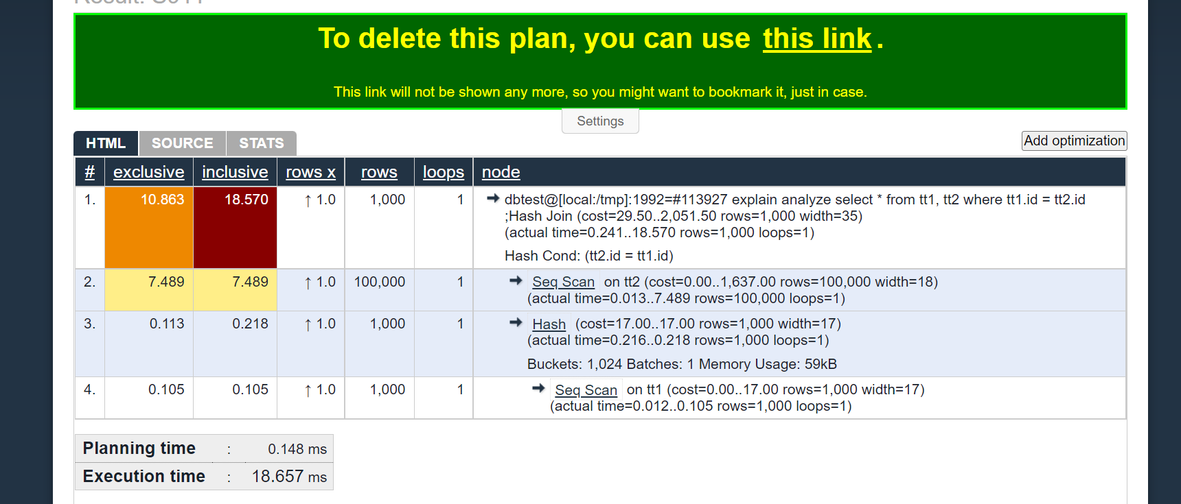
我们可以看到:tt1 作为相对较小的表 在内存 ( Memory Usage: 59kB)中 生成了 1024 hash 桶
dbtest@[local:/tmp]:1992=#113927 explain  analyze select *  from tt1, tt2 where tt1.id = tt2.id ;
                                                   QUERY PLAN
-----------------------------------------------------------------------------------------------------------------
Hash Join  (cost=29.50..2051.50 rows=1000 width=35) (actual time=0.241..18.570 rows=1000 loops=1)
   Hash Cond: (tt2.id = tt1.id)
   ->  Seq Scan on tt2  (cost=0.00..1637.00 rows=100000 width=18) (actual time=0.013..7.489 rows=100000 loops=1)
   ->  Hash  (cost=17.00..17.00 rows=1000 width=17) (actual time=0.216..0.218 rows=1000 loops=1)
         Buckets: 1024  Batches: 1  Memory Usage: 59kB
         ->  Seq Scan on tt1  (cost=0.00..17.00 rows=1000 width=17) (actual time=0.012..0.105 rows=1000 loops=1)
Planning Time: 0.148 ms
Execution Time: 18.657 ms
(8 rows)
最后大家分享一个执行计划可视化的网站: https://explain.depesz.com/
把 explain 出来的文本,复制粘贴到网站中,点击submit 即可得到表格化的图形输出。
Have a fun 🙂 !
