R数据分析|再谈数据标准化、规范化、中心化、对数化

本文主要介绍如何使用datawizard包中的standardise()、normalize()、centre() 三个函数分别进行数据的标准化、规范化和中心化处理。以及多个变量的一次性对数化处理。步骤相较于之前推文R数据分析|数据的标准化、规范化与对数化更为简洁和方便。

0、数据准备

以系统自带的iris数据集为例。主要用到datawizard、tidyverse、bruceR三个包。

install.packages("datawizard")
install.packages("tidyverse")
install.packages("bruceR")
library(datawizard)
library(tidyverse)
library(bruceR)

head(iris)
#  Sepal.Length Sepal.Width Petal.Length Petal.Width Species
#1          5.1         3.5          1.4         0.2  setosa
#2          4.9         3.0          1.4         0.2  setosa
#3          4.7         3.2          1.3         0.2  setosa
#4          4.6         3.1          1.5         0.2  setosa
#5          5.0         3.6          1.4         0.2  setosa
#6          5.4         3.9          1.7         0.4  setosa
iris %>% select(where(is.factor))
iris %>% select(where(is.numeric))

1、标准化

标准化可以将数据转换为均值为0、方差为1的数据。也叫z-score标准化，SPSS中的标准化即为该方法。其公式为：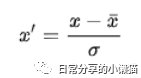

data_stad <- iris %>% select(where(is.numeric)) %>% standardise() #标准化
head(data_stad)
#  Sepal.Length Sepal.Width Petal.Length Petal.Width
#1   -0.8976739  1.01560199    -1.335752   -1.311052
#2   -1.1392005 -0.13153881    -1.335752   -1.311052
#3   -1.3807271  0.32731751    -1.392399   -1.311052
#4   -1.5014904  0.09788935    -1.279104   -1.311052
#5   -1.0184372  1.24503015    -1.335752   -1.311052
#6   -0.5353840  1.93331463    -1.165809   -1.048667
data_stad %>% Describe() #标准化结果，方差为1，均值为0
#Descriptive Statistics:
#──────────────────────────────────────────────────────────────────
#                N  Mean   SD | Median   Min  Max Skewness Kurtosis
#──────────────────────────────────────────────────────────────────
#Sepal.Length  150 -0.00 1.00 |  -0.05 -1.86 2.48     0.31    -0.61
#Sepal.Width   150  0.00 1.00 |  -0.13 -2.43 3.08     0.31     0.14
#Petal.Length  150 -0.00 1.00 |   0.34 -1.56 1.78    -0.27    -1.42
#Petal.Width   150 -0.00 1.00 |   0.13 -1.44 1.71    -0.10    -1.36
#──────────────────────────────────────────────────────────────────

2、规范化

规范化可以将数据的值转换为[0-1]范围内。其公式为：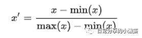

data_norm <- iris %>% select(where(is.numeric)) %>% normalize() #规范化
head(data_norm)
#  Sepal.Length Sepal.Width Petal.Length Petal.Width
#1   0.22222222   0.6250000   0.06779661  0.04166667
#2   0.16666667   0.4166667   0.06779661  0.04166667
#3   0.11111111   0.5000000   0.05084746  0.04166667
#4   0.08333333   0.4583333   0.08474576  0.04166667
#5   0.19444444   0.6666667   0.06779661  0.04166667
#6   0.30555556   0.7916667   0.11864407  0.12500000
data_norm %>% Describe() #规范化，值落在0~1之间
#Descriptive Statistics:
#────────────────────────────────────────────────────────────────
#                N Mean   SD | Median  Min  Max Skewness Kurtosis
#────────────────────────────────────────────────────────────────
#Sepal.Length  150 0.43 0.23 |   0.42 0.00 1.00     0.31    -0.61
#Sepal.Width   150 0.44 0.18 |   0.42 0.00 1.00     0.31     0.14
#Petal.Length  150 0.47 0.30 |   0.57 0.00 1.00    -0.27    -1.42
#Petal.Width   150 0.46 0.32 |   0.50 0.00 1.00    -0.10    -1.36
#────────────────────────────────────────────────────────────────

3、中心化

中心化为各项数据减去均值，可将数据转换为均值为0的数据。其公式为：

data_cent <- iris %>% select(where(is.numeric)) %>% centre() # 中心化
head(data_cent)
#  Sepal.Length Sepal.Width Petal.Length Petal.Width
#1   -0.7433333  0.44266667       -2.358  -0.9993333
#2   -0.9433333 -0.05733333       -2.358  -0.9993333
#3   -1.1433333  0.14266667       -2.458  -0.9993333
#4   -1.2433333  0.04266667       -2.258  -0.9993333
#5   -0.8433333  0.54266667       -2.358  -0.9993333
#6   -0.4433333  0.84266667       -2.058  -0.7993333
data_cent %>% Describe() #中心化结果，均值为0
#Descriptive Statistics:
#──────────────────────────────────────────────────────────────────
#                N  Mean   SD | Median   Min  Max Skewness Kurtosis
#──────────────────────────────────────────────────────────────────
#Sepal.Length  150 -0.00 0.83 |  -0.04 -1.54 2.06     0.31    -0.61
#Sepal.Width   150  0.00 0.44 |  -0.06 -1.06 1.34     0.31     0.14
#Petal.Length  150 -0.00 1.77 |   0.59 -2.76 3.14    -0.27    -1.42
#Petal.Width   150 -0.00 0.76 |   0.10 -1.10 1.30    -0.10    -1.36
#──────────────────────────────────────────────────────────────────

4、对数化

在回归分析的过程中，通常会对数据进行对数化处理，在R可以使用log() 函数（自然对数
）。本文主要介绍如何利用dplyr包中的across() 函数进行多个变量的一次性对数化处理。

data_ln <- iris %>% select(where(is.numeric)) %>% log() # d对数化
head(data_ln)
#  Sepal.Length_ln Sepal.Width_ln Petal.Length_ln Petal.Width_ln
#1        1.629241       1.252763       0.3364722     -1.6094379
#2        1.589235       1.098612       0.3364722     -1.6094379
#3        1.547563       1.163151       0.2623643     -1.6094379
#4        1.526056       1.131402       0.4054651     -1.6094379
#5        1.609438       1.280934       0.3364722     -1.6094379
#6        1.686399       1.360977       0.5306283     -0.9162907
data_cent %>% Describe() #对数化结果
#Descriptive Statistics:
#──────────────────────────────────────────────────────────────────
#                N  Mean   SD | Median   Min  Max Skewness Kurtosis
#──────────────────────────────────────────────────────────────────
#Sepal.Length  150 -0.00 0.83 |  -0.04 -1.54 2.06     0.31    -0.61
#Sepal.Width   150  0.00 0.44 |  -0.06 -1.06 1.34     0.31     0.14
#Petal.Length  150 -0.00 1.77 |   0.59 -2.76 3.14    -0.27    -1.42
#Petal.Width   150 -0.00 0.76 |   0.10 -1.10 1.30    -0.10    -1.36
#──────────────────────────────────────────────────────────────────

5、自定义列进行操作

# 标准化
iris %>% select(Sepal.Length, Sepal.Width) %>% standardise()
# 规范化
iris %>% select(Sepal.Length, Sepal.Width) %>% normalize()
# 中心化
iris %>% select(Sepal.Length, Sepal.Width) %>% centre()
# 对数化
iris %>% select(Sepal.Length, Sepal.Width) %>% log()

6、其他

datawizard包可用于数据塑形，函数功能丰富，更多内容可进一步参考帮助手册^[1]。

如有帮助请多多点赞哦！

参考资料