机器学习概念面试题：ROC-AUC、超参数调优、ZCA Whitening等

原创小小亮 2022-08-26

796

介绍

本数据科学面试系列的前几篇文章讨论了与回归分析、分类指标和集成方法相关的访谈问题。本文将涵盖有关机器学习概念的面试问题，例如 ROC-AUC 曲线和超参数调整。此外，我们将使用所有这些技术及其在Python中的实现。

我们将在本文中使用 Loan Approval 数据集来预测贷款是否已被批准。数据包含 13 列，具有 12 个独立特征和 1 个目标特征，目标变量表示贷款的批准状态，“Y”表示是，“N”表示否。

<strong>Python Code:</strong>
<div class="coding-window"><iframe width="100%" height="1400px" frameborder="no" scrolling="no" sandbox="allow-forms allow-pointer-lock allow-popups allow-same-origin allow-scripts allow-modals" allowfullscreen="allowfullscreen" data-src="https://repl.it/@Santhosh-Reddy1/AUC-ROC?lite=true"><span data-mce-type="bookmark" style="display: inline-block; width: 0px; overflow: hidden; line-height: 0;" class="mce_SELRES_start"></span></iframe></div>

ROC – AUC 曲线

ROC 是描述二元分类器对正类的性能的曲线。它将假阴性率的实际阳性率可视化，突出了模型的敏感性。ROC 曲线在 x 轴上绘制假阳性率，在 y 轴上绘制真阳性率。

真阳性率或灵敏度或召回率是真阳性预测与阳性类别中总真阳性的比率。

TruePositiveRate = TruePositives / (TruePositives + False Negatives)

误报率是误报预测与所有负类示例的比率。

FalsePositiveRate = FalsePositives / (FalsePositives + TrueNegatives)

对于一个完美的模型，我们需要曲线的坐标为 (0, 1)。这意味着正确的正类预测分数为 1，不准确的负类预测为 0。

ROC 曲线为正类和负类之间的截止设置了一个阈值。默认情况下，此阈值设置为 0.5，介于 0 和 1 之间。

通过更改预测平衡，更改阈值会在 TruePositiveRate 和 FalsePositiveRate 之间进行权衡。如果一个指标有所改善，那么另一个指标可能会下降。因此，通过改变阈值，我们可以将 ROC 曲线从左下角延伸到右上角，使其向左上角倾斜 (0, 1)。

此外，我们可以通过查看图来评估分类器是否运行良好。如果图是对角线，则意味着模型无法区分负类和正类。

ROC 曲线在平衡和不平衡的数据集上给出了更好的结果，因为它对更频繁的标签类别没有偏差。

尽管 ROC 曲线似乎是一种有效的模型性能评估器，但有时仅使用曲线比较多个分类器具有挑战性。相反，我们可以使用具有不同阈值的每个模型的 ROC 曲线下面积。该站点是AUC分数，这个评估指标是ROC AUC。得分值介于 0 和 1 之间，其中 1 是满分。

我们已经在 Scikit-Learn 中有一个内置函数来计算 ROC 曲线的 ROC AUC 分数。

让我们在 Python 中实现 ROC AUC 来评估模型预测贷款批准状态的准确度。

y = loan_df['Loan_Status']

X = loan_df.drop(['Loan_ID', 'Loan_Status'], axis = 1)

lbe = LabelEncoder()

y_labeled = lbe.fit_transform(y)

from sklearn.model_selection import train_test_split as tst

X_train, X_valid, y_train, y_valid = tst(X, y_labeled, test_size = 0.25, stratify = y_labeled)

model = LogisticRegression()

model.fit(X_train, y_train)

y_preds = model.predict_proba(X_valid)

from sklearn.metrics import roc_curve

# retrieving just the probabilities for the positive class

pos_probs = y_preds[:, 1]

# plotting no skill roc curve

plt.plot([0, 1], [0, 1], linestyle='--', label='No Skill')

# calculating roc curve for model

fpr, tpr, _ = roc_curve(y_valid, pos_probs)

# plotting model roc curve

plt.plot(fpr, tpr, marker='.', label='Logistic')

# assigning axis labels

plt.xlabel('False Positive Rate')

plt.ylabel('True Positive Rate')

# show the legend

plt.legend()

# show the plot

plt.show()

from sklearn.metrics import roc_auc_score

# calculate roc auc

roc_auc = roc_auc_score(y_valid, pos_probs)

print('Logistic ROC AUC %.3f' % roc_auc)

什么是超参数调优？你能解释一下任何调整方法吗？

我们使用超参数调整技术来获得模型的最佳超参数。超参数是机器学习算法中可用的参数。

有多种技术可以执行超参数调整，我们将通过运行示例讨论每种方法的实现。

让我们首先安装用于 BayesianSearchCV 的 Scikit Optimize 和用于 Xgboost 分类器的 Xgboost。

!pip install scikit_optimize xgboost

from xgboost import XGBClassifier
from sklearn.model_selection import GridSearchCV, RandomizedSearchCV, StratifiedShuffleSplit
from scipy.stats import randint, uniform
from skopt import BayesSearchCV
from skopt.space import Real, Categorical, Integer

GridSearchCV

作为数据科学家，我们经常使用这种方法来获得最佳超参数。此方法使用模型的所有可能超参数排列执行训练。然后我们评估每个排列的性能并选择最佳模型。

由于 GridSearchCV 使用超参数的所有组合，因此计算成本很高。

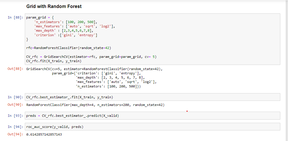
在这个项目中，我们将使用 GridSearchCV 与 Xgboost 和随机森林构建分类模型。

%%time
param = {
    'learning_rate': [.1]
    , 'subsample': [.2, .3 ,.4, .5]
    , 'n_estimators': [25, 50]
    , 'min_child_weight': [25]
    , 'reg_alpha': [.3, .4, .5]
    , 'reg_lambda': [.1, .2, .3, .4, .5]
    , 'colsample_bytree': [.66]
    , 'max_depth': [5]
}
#iter - 4x2x3x5 = 120
model = XGBClassifier(random_state=42, n_jobs=-1) #input hyperparameters without tuning
gridsearch = GridSearchCV(model, param_grid=param, cv=3, n_jobs=-1, scoring='accuracy', return_train_score=True)
gridsearch.fit(X, y_labeled)
print('best score of Grid Search over 120 iterations:', gridsearch.best_score_)

该代码显示了 GridSearchCV 与 Xgboost 分类器的实现。模型构建过程从初始化参数开始，然后 GridSearchCV 通过超参数的排列和组合为 Xgboost 找到最合适的超参数。

随机搜索CV

Randomized SearchCV 使用超参数的列表或统计分布而不是一组离散值，并从分布中随机选择超参数值。

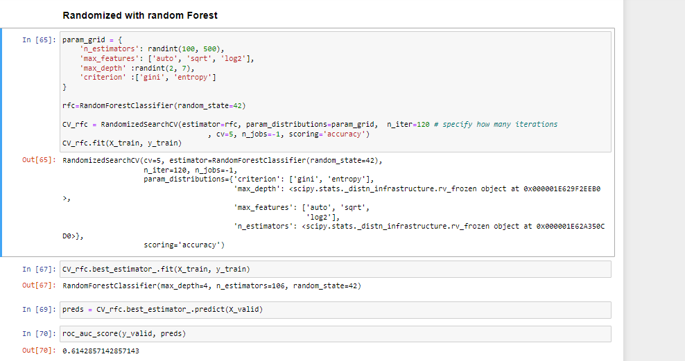
笔记：

GridSearchCV 更适用于小数据集，而对于大数据集，我们应该使用 RandomizedSearchCV 以降低计算复杂度。

%%time
param = {
    'learning_rate': uniform(.05, .1) #actual value: (loc, loc + scale)
    , 'subsample': uniform(.2, .3)
    , 'n_estimators': randint(20, 70)
    , 'min_child_weight': randint(20, 40)
    , 'reg_alpha': uniform(0, .7)
    , 'reg_lambda': uniform(0, .7)
    , 'colsample_bytree': uniform(.1, .7)
    , 'max_depth': randint(2, 6)
}
randomsearch = RandomizedSearchCV(model, param_distributions=param, n_iter=120 # specify how many iterations
                                  , cv=3, n_jobs=-1, scoring='accuracy', return_train_score=True)
randomsearch.fit(X, y_labeled)
print('best score of Randomized Search over 120 iterations:', randomsearch.best_score_)

上面的代码适用于 Xgboost 运行 120 次迭代的随机搜索 CV。第一步是初始化统计分布中的参数，然后使用随机选取的超参数训练模型。

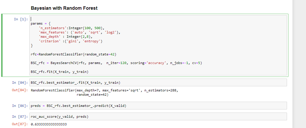
贝叶斯搜索CV

BayasianSearchCV 技术使用贝叶斯优化来探索最适合 ML 模型的超参数。它在采集函数上使用高斯过程回归来最小化采集函数。BayesianSearchcv 跟踪过去的评估结果，并使用它们形成一个概率模型，将超参数映射到目标函数得分的概率。

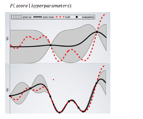
此外，我们可以将广泛的参数值输入贝叶斯优化。因为它会自动探索最合适的区域并丢弃没有希望的区域。

这里的目标函数是使用指定的模型超参数获得最佳预测。

%%time
param = {
    'learning_rate': Real(.05, .1+.05) #lower bound and upper bound
    , 'subsample': Real(.2, .5)
    , 'n_estimators': Integer(20, 70)
    , 'min_child_weight': Integer(20, 40)
    , 'reg_alpha': Real(0, 0+.7)
    , 'reg_lambda': Real(0, 0+.7)
    , 'colsample_bytree': Real(.1, .1+.7)
    , 'max_depth': Integer(2, 6)
}
bayessearch = BayesSearchCV(model, param, n_iter=60, # specify how many iterations
                                    scoring='accuracy', n_jobs=-1, cv=3)
bayessearch.fit(X, y_labeled)
print('best score of Bayes Search over 60 iterations:', bayessearch.best_score_)

该代码用于使用 Xgboost 及其超参数训练 BayesianSearchCV。BayesianSearchCV 使用预定义的超参数范围训练 Xgboost 超过 60 次迭代。BayesianSearchCV 将使用贝叶斯优化确定最佳超参数，同时最小化采集率。

结果：

型号名称	ROC AUC 分数
带有 XGBoost 分类器的 GridSearchCV	0.5
带有 XGBoost 分类器的 RandomizedSearchCV	0.5
带有 XGBoost 分类器的 BayesianSearchCV	0.5

ZCA Whitening 是什么？

ZCA 代表零分量分析，它将协方差矩阵转换为单位矩阵。这个过程从一阶和二阶结构中去除了统计结构。

我们可以使用 ZCA 来驱动彼此线性独立的特征，并将数据转换为零均值。在训练图像分类模型之前，我们可以将 ZCA 白化应用于小彩色图像。该技术用于图像增强以创建更复杂的图片模式，以便模型还可以对模糊和变白的图像进行分类。

我们将尝试实施 ZCA Whitening 以了解使用 Mnist 数据集。

# ZCA Whitening

from tensorflow.keras.datasets import mnist
from tensorflow.keras.preprocessing.image import ImageDataGenerator
import matplotlib.pyplot as plt
# load data
(X_train, y_train), (X_test, y_test) = mnist.load_data()
# reshape to be [samples][width][height][channels]
X_train = X_train.reshape((X_train.shape[0], 28, 28, 1))
X_test = X_test.reshape((X_test.shape[0], 28, 28, 1))
# convert from int to float
X_train = X_train.astype('float32')
X_test = X_test.astype('float32')
# define data preparation
datagen = ImageDataGenerator(featurewise_center=True, featurewise_std_normalization=True, zca_whitening=True)
# fit parameters from data
X_mean = X_train.mean(axis=0)
datagen.fit(X_train - X_mean)
# configure batch size and retrieve one batch of images
for X_batch, y_batch in datagen.flow(X_train - X_mean, y_train, batch_size=9, shuffle=False):
    print(X_batch.min(), X_batch.mean(), X_batch.max())
    # create a grid of 3x3 images
    fig, ax = plt.subplots(3, 3, sharex=True, sharey=True, figsize=(4,4))
    for i in range(3):
        for j in range(3):
            ax[i][j].imshow(X_batch[i*3+j].reshape(28,28), cmap=plt.get_cmap("gray"))
    # show the plot
    plt.show()
    break

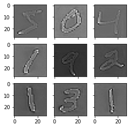
在使用 TensorFlow 和 ImageDatagenerator 应用 ZCA Whitening 后，每张图像的轮廓都已突出显示，如上图所示。

结论

我们已经讨论了一些关于 ZCA Whitening、Hyperparameter Tuning 和 ROC-AUC 的面试问题。我们已经看到，在所有超参数调优技术中，BayesSearchCV 表现良好，ROC AUC 得分为 0.68。

但是，它不能被认为是最终结果。

让我们用一些关键要点来总结博客：

ROC AUC 度量对不平衡分类问题有效。
ROC 曲线绘制了真阳性率与假阴性率的相关性。
AUC 是 ROC 曲线下的面积，当 ROC 曲线结果不可解释时使用。
GridSearchCV 使用所有超参数的排列，因此计算成本很高。
RandomizedSearchCV 从统计分布中选择随机超参数组合。
BayesSearchCV 选择具有贝叶斯优化的超参数。
ZCA Whitening 使特征线性独立，并将数据均值降低到零。
ZCA白化适用于微小的彩色图像，从一阶和二阶统计结构中去除相关性。

原文标题：Data Science Interview Part 3: ROC-AUC
原文作者：Kavish111
原文链接：https://www.analyticsvidhya.com/blog/2022/08/data-science-interview-part-3-roc-auc/

机器学习数据科学墨力翻译

最后修改时间：2022-08-26 10:31:03

「喜欢这篇文章，您的关注和赞赏是给作者最好的鼓励」

关注作者