Fashion-MNIST 服装图片分类-Pytorch实现

大家好，我是小寒。

我们在上一篇文章分享了如何进行手写数字识别。

深度学习案例分享 | 手写数字识别 - PyTorch 实现

读取数据集

# 通过ToTensor实例将图像数据从PIL类型变换成32位浮点数格式，
# 并除以255使得所有像素的数值均在0到1之间
trans = transforms.ToTensor()
mnist_train = torchvision.datasets.FashionMNIST(
            root="../data", train=True, transform=trans, download=True)
mnist_test = torchvision.datasets.FashionMNIST(
            root="../data", train=False, transform=trans, download=True)

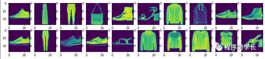
Fashion-MNIST 由10个类别的图像组成，每个类别由训练数据集（train dataset）中的6000张图像和测试数据集（test dataset）中的1000张图像组成。

len(mnist_train), len(mnist_test)

60000,10000

可视化数据集

我们来看一下数据集中的图像样本是什么样的。

通过如下方式，我们来可视化的展示训练集中前几个样本。

# 显示数据集
mnist_show = torchvision.datasets.FashionMNIST(root="../data", train=True, transform=torchvision.transforms.ToTensor(), download=True)
images, label = next(iter(data.DataLoader(mnist_show, 20, shuffle=True)))
images=images.reshape(20,28,28)
fig,axes = plt.subplots(2,10,figsize=(15,3))  
axes = axes.flatten()   
for i, (ax, img) in enumerate(zip(axes, images)):
    if torch.is_tensor(img):
        ax.imshow(img.numpy())
    else:
        # PIL图⽚
        ax.imshow(img)
plt.show()

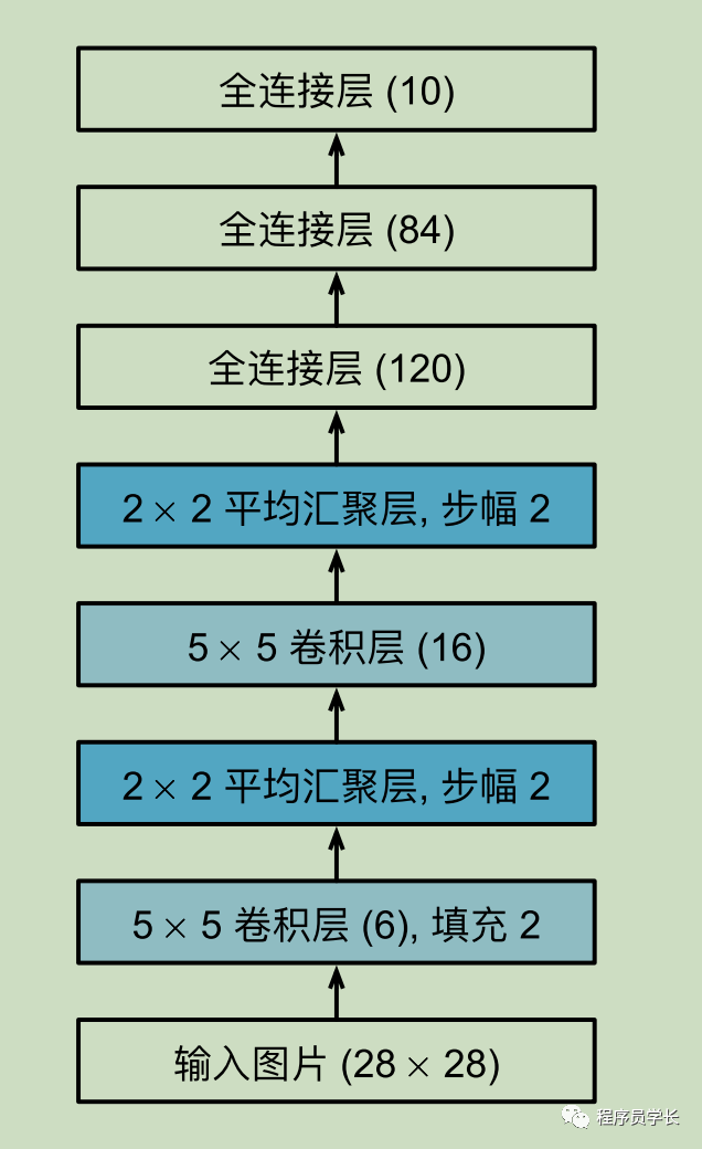
LeNet-5 网络结构

总体来看，LeNet-5 由两个部分组成：

• 两个卷积层。
• 三个全连接层。

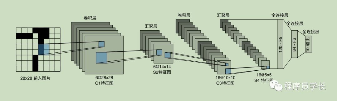
每个卷积块中的基本单元是⼀个卷积层、⼀个 sigmoid 激活函数和平均汇聚层。

每个卷积层使⽤ 5 × 5 卷积核和⼀个 sigmoid 激活函数。

第⼀卷积层有 6 个输出通道，⽽第⼆个卷积层有 16 个输出通道。

下面我们看一下网络结构的定义。

net = nn.Sequential(
        nn.Conv2d(1, 6, kernel_size=5, padding=2), 
        nn.Sigmoid(),
        nn.AvgPool2d(kernel_size=2, stride=2),
        nn.Conv2d(6, 16, kernel_size=5), 
        nn.Sigmoid(),
        nn.AvgPool2d(kernel_size=2, stride=2),
        nn.Flatten(),
        nn.Linear(16 * 5 * 5, 120), 
        nn.Sigmoid(),
        nn.Linear(120, 84), 
        nn.Sigmoid(),
        nn.Linear(84, 10))

X = torch.rand(size=(1, 1, 28, 28), dtype=torch.float32)
for layer in net:
    X = layer(X)
    print(layer.__class__.__name__, 'output shape: \t', X.shape)

输出如下所示：

Conv2d output shape:   torch.Size([1, 6, 28, 28])
Sigmoid output shape:   torch.Size([1, 6, 28, 28])
AvgPool2d output shape:   torch.Size([1, 6, 14, 14])
Conv2d output shape:   torch.Size([1, 16, 10, 10])
Sigmoid output shape:   torch.Size([1, 16, 10, 10])
AvgPool2d output shape:   torch.Size([1, 16, 5, 5])
Flatten output shape:   torch.Size([1, 400])
Linear output shape:   torch.Size([1, 120])
Sigmoid output shape:   torch.Size([1, 120])
Linear output shape:   torch.Size([1, 84])
Sigmoid output shape:   torch.Size([1, 84])
Linear output shape:   torch.Size([1, 10])

初始化模型参数

这里我们使用 「Xavier」 来进行参数的初始化。

def init_weights(m):
    if type(m) == nn.Linear or type(m) == nn.Conv2d:
        nn.init.xavier_uniform_(m.weight)

net.apply(init_weights)

定义损失函数和优化器

#交叉熵作为损失函数
loss = nn.CrossEntropyLoss()
#定义优化器
optimizer = torch.optim.SGD(net.parameters(), lr=0.1)

训练及预测

让我们看看 LeNet-5 在 Fashion-MNIST 数据集上的表现吧。

def train_ch6(net, train_iter, test_iter, num_epochs, lr, device):
    """⽤GPU训练模型"""
    #初始化权重
    def init_weights(m):
        if type(m) == nn.Linear or type(m) == nn.Conv2d:
            nn.init.xavier_uniform_(m.weight)
    net.apply(init_weights)
    print('training on', device)

    #net复制到相应的设备上
    net.to(device)

    #定义优化器
    optimizer = torch.optim.SGD(net.parameters(), lr=lr)
    #交叉熵作为损失函数
    loss = nn.CrossEntropyLoss()
    
    num_batches = len(train_iter)
    train_loss=[]
    train_accs=[]
    starttime = datetime.datetime.now()
    for epoch in range(num_epochs):
        #训练损失之和，训练正确数之和，样本数
        metric = Accumulator(3)
        net.train()
        for i, (X, y) in enumerate(train_iter):
            optimizer.zero_grad()
            X, y = X.to(device), y.to(device)
            y_hat = net(X)
            l = loss(y_hat, y)
            l.backward()
            optimizer.step()
            with torch.no_grad():
                metric.add(l * X.shape[0], accuracy(y_hat, y), X.shape[0])
            #训练损失、训练正确率
            train_l = metric[0] / metric[2]
            train_acc = metric[1] / metric[2]

        train_loss.append(train_l)
        train_accs.append(train_acc)
        print(f'ecoch {epoch+1}, loss {train_l:.3f}, train acc {train_acc:.3f}')

    endtime = datetime.datetime.now()
    time_second= (endtime - starttime).seconds
    print(f'总耗时 {time_second}')
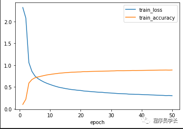
    show_image(num_epochs, train_loss, train_accs)

    test_acc = evaluate_accuracy_gpu(net, test_iter)
    print(f'test acc {test_acc:.3f}')

device = torch.device("cuda:0" if torch.cuda.is_available() else "cpu")
print(device)
lr, num_epochs = 0.5, 50
train_ch6(net, train_iter, test_iter, num_epochs, lr, device)

我们在 GPU 上进行 50 轮的迭代训练，测试集的正确率可以达到89%。

cuda:0
training on cuda:0
ecoch 1, loss 2.320, train acc 0.100
ecoch 2, loss 2.079, train acc 0.219
ecoch 3, loss 1.058, train acc 0.589
ecoch 4, loss 0.859, train acc 0.670
ecoch 5, loss 0.751, train acc 0.709
ecoch 6, loss 0.691, train acc 0.729
ecoch 7, loss 0.648, train acc 0.746
ecoch 8, loss 0.611, train acc 0.762
ecoch 9, loss 0.581, train acc 0.777
ecoch 10, loss 0.556, train acc 0.786
ecoch 11, loss 0.531, train acc 0.797
ecoch 12, loss 0.510, train acc 0.806
ecoch 13, loss 0.491, train acc 0.815
ecoch 14, loss 0.478, train acc 0.821
ecoch 15, loss 0.463, train acc 0.827
ecoch 16, loss 0.452, train acc 0.832
ecoch 17, loss 0.441, train acc 0.837
ecoch 18, loss 0.434, train acc 0.839
ecoch 19, loss 0.425, train acc 0.843
ecoch 20, loss 0.420, train acc 0.845
ecoch 21, loss 0.408, train acc 0.851
ecoch 22, loss 0.403, train acc 0.851
ecoch 23, loss 0.396, train acc 0.855
...
ecoch 48, loss 0.303, train acc 0.888
ecoch 49, loss 0.305, train acc 0.886
ecoch 50, loss 0.300, train acc 0.889
总耗时 378
test acc 0.890

最后