R语言绘图|气泡地图

上一期介绍了如何利用ggplot2绘制分级颜色填充地图，本期接上期内容继续介绍如何利用ggplot2绘制气泡形式的填充地图，具体下图所示：

1、绘图

library(tmap)
library(sf)
library(see)
library(dplyr)
library(viridis)
library(ggplot2)
World <- data("World")
countries <- World %>% filter(continent == "Africa") #提取Africa地理信息
countries
#Simple feature collection with 51 features and 15 fields
#Geometry type: MULTIPOLYGON
#Dimension:     XY
#Bounding box:  xmin: -17.62504 ymin: -34.81917 xmax: 51.13387 ymax: 37.34999
#Geodetic CRS:  WGS 84
countries.point <- st_centroid(countries, of_largest_polygon = TRUE) #convert to 
#绘图
ggplot() + 
  geom_sf(data = countries) +  
  geom_sf(data = countries.point, aes(size = gdp_cap_est)) + 
  theme_minimal()

2、修改填充颜色及映射

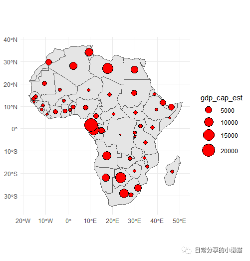
1.修改填充颜色

ggplot() + 
  geom_sf(data = countries) +  
  geom_sf(data = countries.point,shape = 21, aes(size = gdp_cap_est), fill = "red") + 
  scale_size_continuous(range = c(1, 9)) + 
  theme_minimal()

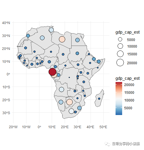
2.加入fill映射

ggplot() + 
  geom_sf(data = countries) +  
  geom_sf(data = countries.point,shape = 21, aes(size = gdp_cap_est, fill = gdp_cap_est)) + 
  scale_fill_distiller(palette = "RdBu") + 
  scale_size_continuous(range = c(1, 9)) + 
  theme_minimal()

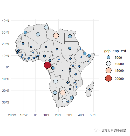
3.合并size与fill映射图例

ggplot() + #合并图例
  geom_sf(data = countries) +  
  geom_sf(data = countries.point,shape = 21, aes(size = gdp_cap_est, fill = gdp_cap_est)) + 
  scale_fill_distiller(palette = "RdBu") + 
  scale_size_continuous(range = c(1, 9)) + 
  theme_minimal() + 
  guides(fill = guide_legend(), size = guide_legend())

3、其他

关于ggplot2绘制颜色绘制可参考R语言绘图|色彩填充地图。关于Python绘制地图可参考Python空间分析|分级颜色地图绘制，tmap包绘制地图可参考R语言绘图 | 利用tmap绘制分级色彩地图。更多绘图方法可进一步阅读公众号其他文章。

如有帮助请多多点赞哦！