R语言广义线性模型GLM、多项式回归和广义可加模型GAM预测泰坦尼克号幸存者

拓端数据部落 2022-09-28

343

全文下载链接：http://tecdat.cn/?p=18266

本文通过R语言建立广义线性模型(GLM)、多项式回归和广义可加模型（GAM）来预测谁在1912年的泰坦尼克号沉没中幸存下来。

相关视频

                       拓端该视频号动态不可引用
str(titanic)

数据变量为：

Survived
：乘客存活指标（如果存活则为1）
Pclass
：旅客舱位等级
Sex
：乘客性别
Age
：乘客年龄
SibSp
：兄弟姐妹/配偶人数
Parch
：父母/子女人数
Embarked
：登船港口
Name
：旅客姓名

最后一个变量使用不多，因此我们将其删除，

titanic = titanic[,1:7]

现在，我们回答问题：

幸存的旅客比例是多少？

简单的答案是





mean(titanic$Survived)
[1] 0.3838384

可以在下面的列联表中找到





table(titanic$Survived)/nrow(titanic)
0         1
0.6161616 0.3838384

或此处幸存者的38.38 ％。也就是说，也可以通过不对任何解释变量进行逻辑回归来获得（换句话说，仅对常数进行回归）。回归给出了：









Coefficients:
(Intercept)
-0.4733




Degrees of Freedom: 890 Total (i.e. Null);  890 Residual
Null Deviance:      1187
Residual Deviance: 1187   AIC: 1189

给出β0的值，并且由于生存概率为

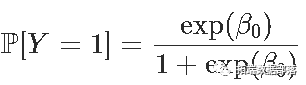
我们通过考虑



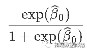
exp(-0.4733)/(1+exp(-0.4733))
[1] 0.3838355

我们也可以使用predict
函数





predict(glm(Survived~1, family=binomial,type="response")[1]
1
0.3838384

此外，在概率回归中也适用，





reg=glm(Survived~1, family=binomial(link="probit"),data=titanic)
predict(reg,type="response")[1]
1
0.3838384

幸存的头等舱乘客的比例是多少？

我们只看头等舱的人，

[1] 0.6296296

约63％存活。我们可以进行逻辑回归







Coefficients:
(Intercept)      Pclass2      Pclass3
0.5306      -0.6394      -1.6704




Degrees of Freedom: 890 Total (i.e. Null);  888 Residual
Null Deviance:      1187
Residual Deviance: 1083   AIC: 1089

由于第1类是参考类，因此我们照旧考虑





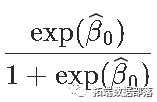
exp(0.5306)/(1+exp(0.5306))
[1] 0.629623

predict预测：









predict(reg,newdata=data.frame(Pclass="1"),type="response")
1
0.6296296

我们可以尝试概率回归，我们得到的结果是一样的，









predict(reg,newdata=data.frame(Pclass="1"),type="response")
1
0.6296296

卡方独立性测试：在生存与否之间的检验统计量是多少？

卡方检验的命令如下



chisq.test(table( Survived, Pclass))




Pearson's Chi-squared test




data:  table( Survived,  Pclass)
X-squared = 102.89, df = 2, p-value &lt; 2.2e-16

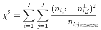
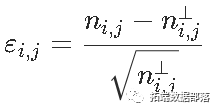
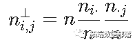
我们有一个列联表，如果变量是独立的，我们有，然后是统计量，我们可以看到，对测试的贡献





1         2         3
0 -4.601993 -1.537771  3.993703
1  5.830678  1.948340 -5.059981

这给了我们很多信息：我们观察到两个正值，分别对应于“幸存”和“头等舱”与“无法幸存”和“三等舱”之间的强（正）关联，以及两个很强的负值，对应于“生存”和“第三等”之间的强烈负相关，以及“无法幸存”和“头等舱”。我们可以在下图上可视化这些值





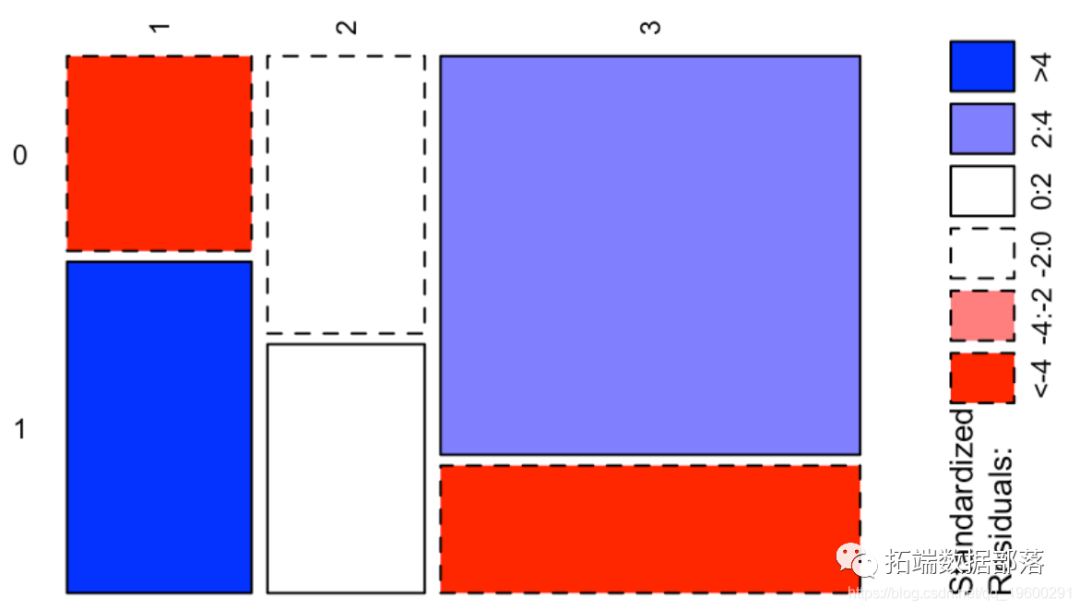
ass(table( Survived, Pclass), shade = TRUE, las=3)

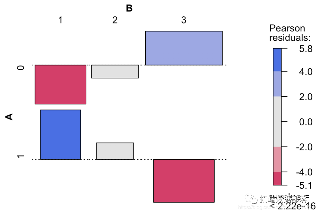
然后我们必须进行逻辑回归，并预测两名模拟乘客的生存概率

点击标题查阅往期内容

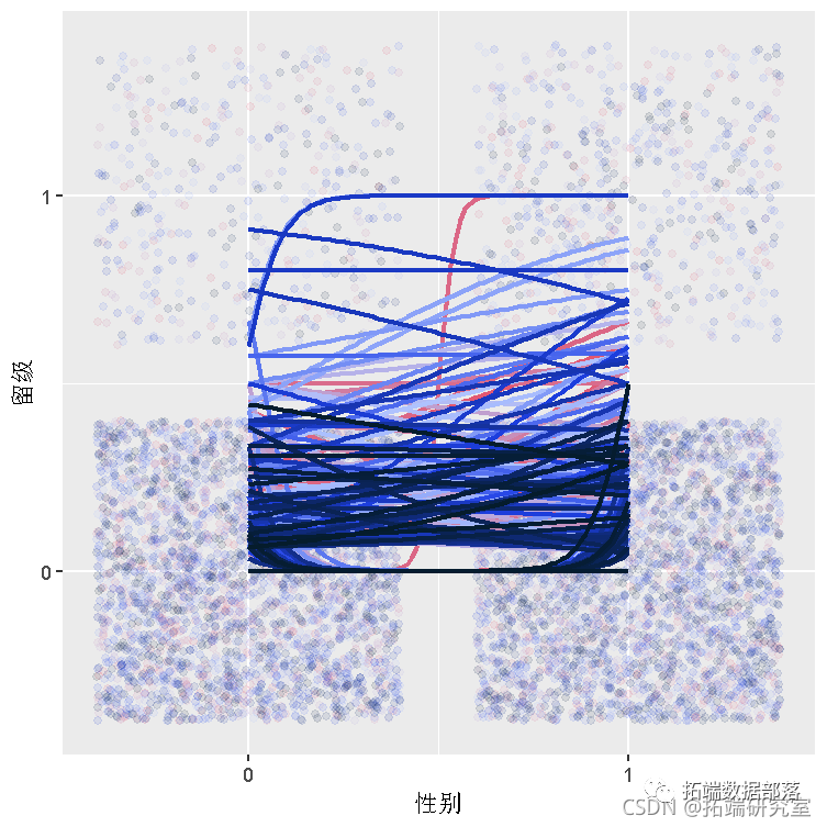
R语言贝叶斯广义线性混合（多层次/水平/嵌套）模型GLMM、逻辑回归分析教育留级影响因素数据

左右滑动查看更多

假设我们有两名乘客



newbase = data.frame(
Pclass = as.factor(c(1,3)),
Sex = as.factor(c("female","male")),
Age = c(17,20),
SibSp = c(1,0),
Parch = c(2,0),

让我们对所有变量进行简单回归，













Coefficients:
Estimate Std. Error z value Pr(&gt;|z|)
(Intercept)  16.830381 607.655774   0.028  0.97790
Pclass2      -1.268362   0.298428  -4.250 2.14e-05 ***
Pclass3      -2.493756   0.296219  -8.419  &lt; 2e-16 ***
Sexmale      -2.641145   0.222801 -11.854  &lt; 2e-16 ***
Age          -0.043725   0.008294  -5.272 1.35e-07 ***
SibSp        -0.355755   0.128529  -2.768  0.00564 **
Parch        -0.044628   0.120705  -0.370  0.71159
EmbarkedC   -12.260112 607.655693  -0.020  0.98390
EmbarkedQ   -13.104581 607.655894  -0.022  0.98279
EmbarkedS   -12.687791 607.655674  -0.021  0.98334
---
Signif. codes:  0 ‘***’ 0.001 ‘**’ 0.01 ‘*’ 0.05 ‘.’ 0.1 ‘ ’ 1




(Dispersion parameter for binomial family taken to be 1)




Null deviance: 964.52  on 713  degrees of freedom
Residual deviance: 632.67  on 704  degrees of freedom
(177 observations deleted due to missingness)
AIC: 652.67




Number of Fisher Scoring iterations: 13

两个变量并不重要。我们删除它们













Coefficients:
Estimate Std. Error z value Pr(&gt;|z|)
(Intercept)  4.334201   0.450700   9.617  &lt; 2e-16 ***
Pclass2     -1.414360   0.284727  -4.967 6.78e-07 ***
Pclass3     -2.652618   0.285832  -9.280  &lt; 2e-16 ***
Sexmale     -2.627679   0.214771 -12.235  &lt; 2e-16 ***
Age         -0.044760   0.008225  -5.442 5.27e-08 ***
SibSp       -0.380190   0.121516  -3.129  0.00176 **
---
Signif. codes:  0 ‘***’ 0.001 ‘**’ 0.01 ‘*’ 0.05 ‘.’ 0.1 ‘ ’ 1




(Dispersion parameter for binomial family taken to be 1)




Null deviance: 964.52  on 713  degrees of freedom
Residual deviance: 636.56  on 708  degrees of freedom
(177 observations deleted due to missingness)
AIC: 648.56




Number of Fisher Scoring iterations: 5

我们有年龄这样的连续变量时，我们可以进行多项式回归













Coefficients:
Estimate Std. Error z value Pr(&gt;|z|)
(Intercept)     3.0213     0.2903  10.408  &lt; 2e-16 ***
Pclass2        -1.3603     0.2842  -4.786 1.70e-06 ***
Pclass3        -2.5569     0.2853  -8.962  &lt; 2e-16 ***
Sexmale        -2.6582     0.2176 -12.216  &lt; 2e-16 ***
poly(Age, 3)1 -17.7668     3.2583  -5.453 4.96e-08 ***
poly(Age, 3)2   6.0044     3.0021   2.000 0.045491 *
poly(Age, 3)3  -5.9181     3.0992  -1.910 0.056188 .
SibSp          -0.5041     0.1317  -3.828 0.000129 ***
---
Signif. codes:  0 ‘***’ 0.001 ‘**’ 0.01 ‘*’ 0.05 ‘.’ 0.1 ‘ ’ 1




(Dispersion parameter for binomial family taken to be 1)




Null deviance: 964.52  on 713  degrees of freedom
Residual deviance: 627.55  on 706  degrees of freedom
AIC: 643.55




Number of Fisher Scoring iterations: 5

但是解释参数变得很复杂。我们注意到三阶项在这里很重要，因此我们将手动进行回归









Coefficients:
Estimate Std. Error z value Pr(&gt;|z|)
(Intercept)  5.616e+00  6.565e-01   8.554  &lt; 2e-16 ***
Pclass2     -1.360e+00  2.842e-01  -4.786  1.7e-06 ***
Pclass3     -2.557e+00  2.853e-01  -8.962  &lt; 2e-16 ***
Sexmale     -2.658e+00  2.176e-01 -12.216  &lt; 2e-16 ***
Age         -1.905e-01  5.528e-02  -3.446 0.000569 ***
I(Age^2)     4.290e-03  1.854e-03   2.314 0.020669 *
I(Age^3)    -3.520e-05  1.843e-05  -1.910 0.056188 .
SibSp       -5.041e-01  1.317e-01  -3.828 0.000129 ***
---
Signif. codes:  0 ‘***’ 0.001 ‘**’ 0.01 ‘*’ 0.05 ‘.’ 0.1 ‘ ’ 1




(Dispersion parameter for binomial family taken to be 1)




Null deviance: 964.52  on 713  degrees of freedom
Residual deviance: 627.55  on 706  degrees of freedom
AIC: 643.55




Number of Fisher Scoring iterations: 5

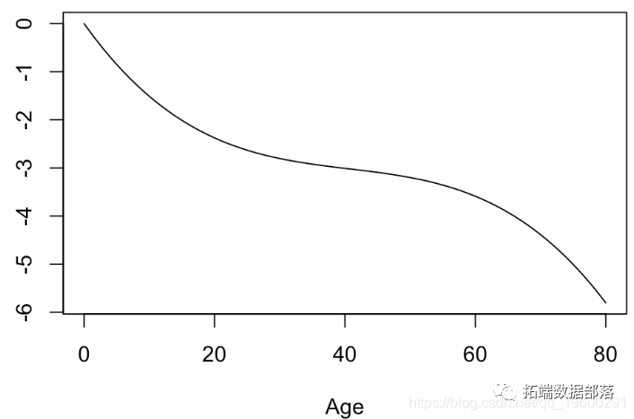
可以看到，p值是相同的。简而言之，将年龄转换为年龄的非线性函数是有意义的。可以可视化此函数









plot(xage,yage,xlab="Age",ylab="",type="l")

实际上，我们可以使用样条曲线。广义可加模型（ gam ）是完美的可视化工具











(Dispersion Parameter for binomial family taken to be 1)




Null Deviance: 964.516 on 713 degrees of freedom
Residual Deviance: 627.5525 on 706 degrees of freedom
AIC: 643.5525
177 observations deleted due to missingness




Number of Local Scoring Iterations: 4




Anova for Parametric Effects
Df Sum Sq Mean Sq  F value    Pr(&gt;F)
Pclass      2  26.72  13.361  11.3500 1.407e-05 ***
Sex         1 131.57 131.573 111.7678 &lt; 2.2e-16 ***
bs(Age)     3  22.76   7.588   6.4455 0.0002620 ***
SibSp       1  14.66  14.659  12.4525 0.0004445 ***
Residuals 706 831.10   1.177
---
Signif. codes:  0 ‘***’ 0.001 ‘**’ 0.01 ‘*’ 0.05 ‘.’ 0.1 ‘ ’ 1

我们可以看到年龄变量的变换，

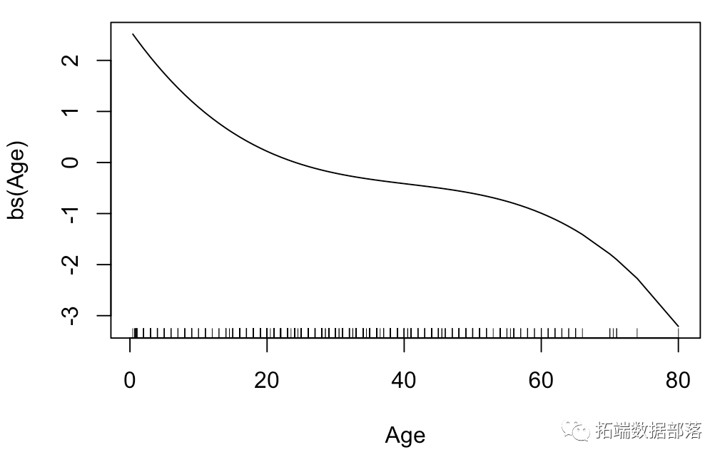
并且我们发现变换接近于我们的3阶多项式。我们可以添加置信带，从而可以验证该函数不是真正的线性

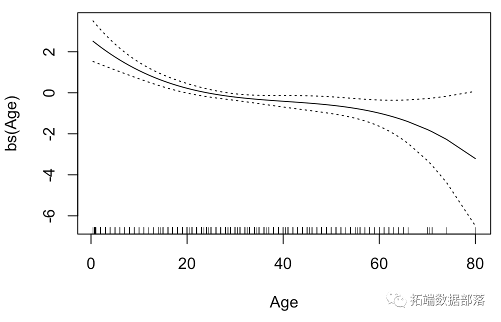
我们现在有三个模型。最后给出了两个模拟乘客的预测，



predict(reg,newdata=newbase,type="response")
1         2
0.9605736 0.1368988
predict(reg3,newdata=newbase,type="response")
1         2
0.9497834 0.1218426
predict(regam,newdata=newbase,type="response")
1         2
0.9497834 0.1218426