


1. 公众号回复0615即可获得下载地址。
2. 为了支持我得学城,欢迎转发,感谢!
全文约3500字,预计阅读时间9分钟。

前置说明
应用场景
配置环境及安装
conda create -n pygeo38 python=3.8
conda activate pygeo38
conda install -c conda-forge geopandas rasterio -y
conda install ipykernel rasterstats -y
python -m ipykernel install --user --name pygeo38 --display-name "GeoPython 3.8成功后进入该环境进行后续实践。
conda activate pygeo38
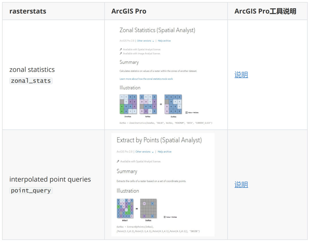
与ArcGIS的对应关系

数据格式支持
栅格 Raster
矢量 Vector

可进行的统计类型
默认
其他可用
自定统计方法

基础使用
区域统计
from rasterstats import zonal_stats
zonal_stats(
"polygons.shp",
# Polygon矢量文件路径
"elevation.tif",
# 栅格文件路径
stats="count min mean max" # 统计类型 详见上节
)返回值为包含相应结果的列表对象,可用Pandas转为
DataFrame对象。
[{'count':75,
'max':22.273418426513672,
'mean':14.660084635416666,
'min':6.575114727020264},
{'count':50,
'max':82.69043731689453,
'mean':56.60576171875,
'min':16.940950393676758}]
点查询 from rasterstats import point_query
point_query(
"polygons.shp", # Points矢量文件路径
"elevation.tif", # 栅格文件路径
)返回值为包含相应结果的列表对象。

基础使用实例——格网统计重庆市平均高程
导入相关库
from pathlib import Path # 处理文件路径
import rasterio as rio
from rasterio.plot import show
from shapely.geometry import box
from rasterstats import zonal_stats
data_path = Path('./data')
dem_file = data_path  "dem.tif"
boundary_file = data_path  "重庆市界.shp"
gdf = gpd.read_file(boundary_file, encoding='gbk')查看原始数据
ax = gdf.plot(facecolor='none', edgecolor='red')
with rio.open(dem_file) as f:
    show(f, cmap='terrain', ax=ax)
gdf.crs

# 确定是投影坐标系
<Projected CRS: EPSG:32648>
Name: WGS 84  UTM zone 48N
Axis Info [cartesian]:
- E[east]: Easting (metre)
- N[north]: Northing (metre)
Area of Use:
- name: World - N hemisphere - 102°E to 108°E - by country
- bounds: (102.0, 0.0, 108.0, 84.0)
Coordinate Operation:
- name: UTM zone 48N
- method: Transverse Mercator
Datum: World Geodetic System 1984
- Ellipsoid: WGS 84
- Prime Meridian: Greenwich创建5km网格
# 获取做500m缓冲区后的外轮廓的外包矩形的四角坐标
cell_width = 5000  # 网格边长
minx, miny, maxx, maxy = gdf.buffer(cell_width  2).bounds.values[0]
# 获取每个小方格的左下角坐标
xmin_lst = np.arange(minx // cell_width, maxx // cell_width, 1) * cell_width
ymin_lst = np.arange(miny // cell_width, maxy // cell_width, 1) * cell_width
# 生成矩阵
x1, y1 = np.meshgrid(xmin_lst, ymin_lst)
# 获取右上角坐标
x2 = x1 + cell_width
y2 = y1 + cell_width
x1, y1, x2, y2 = [i.flatten() for iin [x1, y1, x2, y2]]
# 生成网格
boxes = [box(*i) for i in zip(x1, y1, x2, y2)]
gdf_fishnet = gpd.GeoDataFrame(geometry=boxes, crs=gdf.crs).reset_index()
# 存为shapefile
gdf_fishnet.to_file(data_path / 'fishnet.shp')
gdf_fishnet.shape
(8554, 2)
f, ax = plt.subplots(1,1, figsize=(10,10))
gdf.plot(facecolor='none', edgecolor='red', ax=ax)
with rio.open(dem_file) as f:
    show(f, cmap='terrain', ax=ax)

gdf_fishnet.plot(facecolor='none', edgecolor='blue', ax=ax,lw=0.3)

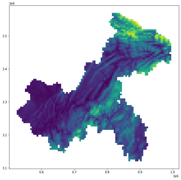
区域统计
stat_result = zonal_stats(
    (data_path /'fishnet.shp').__str__(),

# 无法识别pathlib的类型 转为字符串 也可以直接使用相对路径和绝对路径
    (data_path /'dem.tif').__str__()
    stats="count min mean max"
)
gdf_result = gdf_fishnet.join(pd.DataFrame(stat_result))
gdf_result.plot(column='mean', figsize=(10,10))
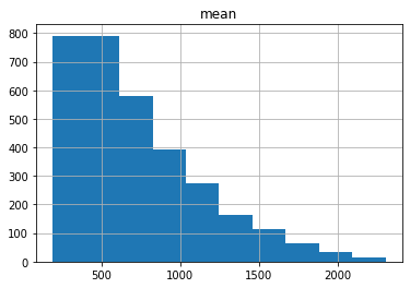
gdf_result = gdf_result[gdf_result['count']>200]
gdf_result.hist(column='mean')

结语
1. 科研论文中的技术方法,比如论文中的关键技术;
2. 机器学习与深度学习算法原理,比如像之前介绍PCA与K-means原理的文章;
3. 机器学习与深度学习在科研与业务中的应用,这是后面关注的重点,会有很多文章,敬请期待;
4. 学术论文写作方法与技巧,后面会请学术大咖做客我得学城,介绍论文写作方法与技巧;
5. 业务咨询类的量化分析技术,比如国土空间规划中的相关量化方法与技术。
文章转载自我得学城,如果涉嫌侵权,请发送邮件至:contact@modb.pro进行举报,并提供相关证据,一经查实,墨天轮将立刻删除相关内容。
