


原文链接:http://tecdat.cn/?p=6145
在本文中,我们用SAS进行泊松,零膨胀泊松和有限混合Poisson模型分析(点击文末“阅读原文”获取完整代码数据)。
泊松模型
proc fmm data = tmp1 tech = trureg;

  model majordrg = age acadmos minordrg logspend  dist = truncpoisson;


  probmodel age acadmos minordrg logspend;


/*

Fit Statistics


-2 Log Likelihood             8201.0

AIC  (smaller is better)      8221.0

AICC (smaller is better)      8221.0

BIC  (smaller is better)      8293.5


Parameter Estimates for 'Truncated Poisson' Model


                                Standard

Component  Effect     Estimate     Error  z Value  Pr > |z|


        1  Intercept   -2.0706    0.3081    -6.72    <.0001

        1  AGE         0.01796  0.005482     3.28    0.0011

        1  ACADMOS    0.000852  0.000700     1.22    0.2240

        1  MINORDRG     0.1739   0.03441     5.05    <.0001

        1  LOGSPEND     0.1229   0.04219     2.91    0.0036


Parameter Estimates for Mixing Probabilities


                         Standard

Effect       Estimate       Error    z Value    Pr > |z|


Intercept     -4.2309      0.1808     -23.40      <.0001

AGE           0.01694    0.003323       5.10      <.0001

ACADMOS      0.002240    0.000492       4.55      <.0001

MINORDRG       0.7653     0.03842      19.92      <.0001

LOGSPEND       0.2301     0.02683       8.58      <.0001

*/


*** HURDLE POISSON MODEL WITH NLMIXED PROCEDURE ***;

proc nlmixed data = tmp1 tech = trureg maxit = 500;

  parms B1_intercept = -4 B1_age = 0 B1_acadmos = 0 B1_minordrg = 0 B1_logspend = 0

        B2_intercept = -2 B2_age = 0 B2_acadmos = 0 B2_minordrg = 0 B2_logspend = 0;


  eta1 = B1_intercept + B1_age * age + B1_acadmos * acadmos + B1_minordrg * minordrg + B1_logspend * logspend;

  exp_eta1 = exp(eta1);

  p0 = 1  (1 + exp_eta1);

  eta2 = B2_intercept + B2_age * age + B2_acadmos * acadmos + B2_minordrg * minordrg + B2_logspend * logspend;

  exp_eta2 = exp(eta2);

  if majordrg = 0 then _prob_ = p0;

  else _prob_ = (1 - p0) * exp(-exp_eta2) * (exp_eta2 ** majordrg)  ((1 - exp(-exp_eta2)) * fact(majordrg));

  ll = log(_prob_);

  model majordrg ~ general(ll);

run;

/*

Fit Statistics


-2 Log Likelihood                 8201.0

AIC (smaller is better)           8221.0

AICC (smaller is better)          8221.0

BIC (smaller is better)           8293.5


Parameter Estimates


                          Standard

Parameter      Estimate      Error     DF   t Value   Pr > |t|


B1_intercept    -4.2309     0.1808    1E4    -23.40     <.0001

B1_age          0.01694   0.003323    1E4      5.10     <.0001

B1_acadmos     0.002240   0.000492    1E4      4.55     <.0001

B1_minordrg      0.7653    0.03842    1E4     19.92     <.0001

B1_logspend      0.2301    0.02683    1E4      8.58     <.0001

============

B2_intercept    -2.0706     0.3081    1E4     -6.72     <.0001

B2_age          0.01796   0.005482    1E4      3.28     0.0011

B2_acadmos     0.000852   0.000700    1E4      1.22     0.2240

B2_minordrg      0.1739    0.03441    1E4      5.05     <.0001

B2_logspend      0.1229    0.04219    1E4      2.91     0.0036

*/
零膨胀泊松模型
*** ZERO-INFLATED POISSON MODEL WITH FMM PROCEDURE ***;

proc fmm data = tmp1 tech = trureg;

  model majordrg = age acadmos minordrg logspend  dist = poisson;


  probmodel age acadmos minordrg logspend;

run;

/*

Fit Statistics


-2 Log Likelihood             8147.9

AIC  (smaller is better)      8167.9

AICC (smaller is better)      8167.9

BIC  (smaller is better)      8240.5


Parameter Estimates for 'Poisson' Model


                                Standard

Component  Effect     Estimate     Error  z Value  Pr > |z|


        1  Intercept   -2.2780    0.3002    -7.59    <.0001

        1  AGE         0.01956  0.006019     3.25    0.0012

        1  ACADMOS    0.000249  0.000668     0.37    0.7093

        1  MINORDRG     0.1176   0.02711     4.34    <.0001

        1  LOGSPEND     0.1644   0.03531     4.66    <.0001


Parameter Estimates for Mixing Probabilities


                         Standard

Effect       Estimate       Error    z Value    Pr > |z|


Intercept     -1.9111      0.4170      -4.58      <.0001

AGE          -0.00082    0.008406      -0.10      0.9218

ACADMOS      0.002934    0.001085       2.70      0.0068

MINORDRG       1.4424      0.1361      10.59      <.0001

LOGSPEND      0.09562     0.05080       1.88      0.0598

*/


*** ZERO-INFLATED POISSON MODEL WITH NLMIXED PROCEDURE ***;

proc nlmixed data = tmp1 tech = trureg maxit = 500;

  parms B1_intercept = -2 B1_age = 0 B1_acadmos = 0 B1_minordrg = 0 B1_logspend = 0

        B2_intercept = -2 B2_age = 0 B2_acadmos = 0 B2_minordrg = 0 B2_logspend = 0;


  eta1 = B1_intercept + B1_age * age + B1_acadmos * acadmos + B1_minordrg * minordrg + B1_logspend * logspend;

  exp_eta1 = exp(eta1);

  p0 = 1  (1 + exp_eta1);

  eta2 = B2_intercept + B2_age * age + B2_acadmos * acadmos + B2_minordrg * minordrg + B2_logspend * logspend;

  exp_eta2 = exp(eta2);

  if majordrg = 0 then _prob_ = p0 + (1 - p0) * exp(-exp_eta2);

  else _prob_ = (1 - p0) * exp(-exp_eta2) * (exp_eta2 ** majordrg)  fact(majordrg);

  ll = log(_prob_);

  model majordrg ~ general(ll);

run;

/*

Fit Statistics


-2 Log Likelihood                 8147.9

AIC (smaller is better)           8167.9

AICC (smaller is better)          8167.9

BIC (smaller is better)           8240.5


Parameter Estimates


                          Standard

Parameter      Estimate      Error     DF   t Value   Pr > |t|


B1_intercept    -1.9111     0.4170    1E4     -4.58     <.0001

B1_age         -0.00082   0.008406    1E4     -0.10     0.9219

B1_acadmos     0.002934   0.001085    1E4      2.70     0.0068

B1_minordrg      1.4424     0.1361    1E4     10.59     <.0001

B1_logspend     0.09562    0.05080    1E4      1.88     0.0598

============

B2_intercept    -2.2780     0.3002    1E4     -7.59     <.0001

B2_age          0.01956   0.006019    1E4      3.25     0.0012

B2_acadmos     0.000249   0.000668    1E4      0.37     0.7093

B2_minordrg      0.1176    0.02711    1E4      4.34     <.0001

B2_logspend      0.1644    0.03531    1E4      4.66     <.0001

*/
点击标题查阅往期内容

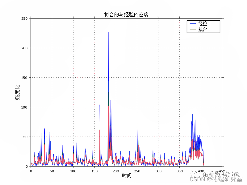
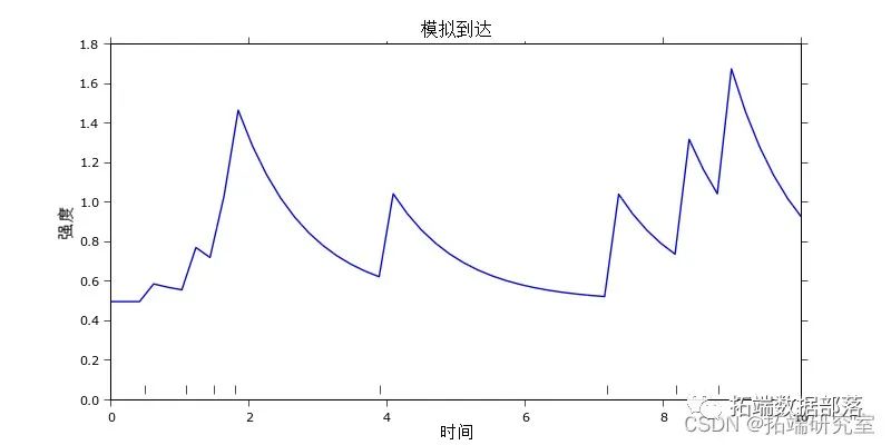
R语言和Python用泊松过程扩展:霍克斯过程Hawkes Processes分析比特币交易数据订单到达自激过程时间序列

左右滑动查看更多


两类有限混合Poisson模型
*** TWO-CLASS FINITE MIXTURE POISSON MODEL WITH FMM PROCEDURE ***;

proc fmm data = tmp1 tech = trureg;

  model majordrg = age acadmos minordrg logspend  dist = poisson k = 2;


run;

/*

Fit Statistics


-2 Log Likelihood             8136.8

AIC  (smaller is better)      8166.8

AICC (smaller is better)      8166.9

BIC  (smaller is better)      8275.7


Parameter Estimates for 'Poisson' Model


                                Standard

Component  Effect     Estimate     Error  z Value  Pr > |z|


        1  Intercept   -2.4449    0.3497    -6.99    <.0001

        1  AGE         0.02214  0.006628     3.34    0.0008

        1  ACADMOS    0.000529  0.000770     0.69    0.4920

        1  MINORDRG    0.05054   0.04015     1.26    0.2081

        1  LOGSPEND     0.2140   0.04127     5.18    <.0001

        2  Intercept   -8.0935    1.5915    -5.09    <.0001

        2  AGE         0.01150   0.01294     0.89    0.3742

        2  ACADMOS    0.004567  0.002055     2.22    0.0263

        2  MINORDRG     0.2638    0.6770     0.39    0.6968

        2  LOGSPEND     0.6826    0.2203     3.10    0.0019


Parameter Estimates for Mixing Probabilities


                         Standard

Effect       Estimate       Error    z Value    Pr > |z|


Intercept     -1.4275      0.5278      -2.70      0.0068

AGE          -0.00277     0.01011      -0.27      0.7844

ACADMOS      0.001614    0.001440       1.12      0.2623

MINORDRG       1.5865      0.1791       8.86      <.0001

LOGSPEND     -0.06949     0.07436      -0.93      0.3501

*/


*** TWO-CLASS FINITE MIXTURE POISSON MODEL WITH NLMIXED PROCEDURE ***;

proc nlmixed data = tmp1 tech = trureg maxit = 500;


        B2_intercept = -8 B2_age = 0 B2_acadmos = 0 B2_minordrg = 0 B2_logspend = 0


  eta1 = B1_intercept + B1_age * age + B1_acadmos * acadmos + B1_minordrg * minordrg + B1_logspend * logspend;

  exp_eta1 = exp(eta1);

  prob1 = exp(-exp_eta1) * exp_eta1 ** majordrg  fact(majordrg);

  eta2 = B2_intercept + B2_age * age + B2_acadmos * acadmos + B2_minordrg * minordrg + B2_logspend * logspend;

  exp_eta2 = exp(eta2);

  prob2 = exp(-exp_eta2) * exp_eta2 ** majordrg  fact(majordrg);

  eta3 = B3_intercept + B3_age * age + B3_acadmos * acadmos + B3_minordrg * minordrg + B3_logspend * logspend;

  exp_eta3 = exp(eta3);

  p = exp_eta3  (1 + exp_eta3);

  _prob_ = p * prob1 + (1 - p) * prob2;

  ll = log(_prob_);

  model majordrg ~ general(ll);

run;

/*

Fit Statistics


-2 Log Likelihood                 8136.8

AIC (smaller is better)           8166.8

AICC (smaller is better)          8166.9

BIC (smaller is better)           8275.7


Parameter Estimates


                          Standard

Parameter      Estimate      Error     DF   t Value   Pr > |t|


B1_intercept    -2.4449     0.3497    1E4     -6.99     <.0001

B1_age          0.02214   0.006628    1E4      3.34     0.0008

B1_acadmos     0.000529   0.000770    1E4      0.69     0.4920

B1_minordrg     0.05054    0.04015    1E4      1.26     0.2081

B1_logspend      0.2140    0.04127    1E4      5.18     <.0001

============

B2_intercept    -8.0935     1.5916    1E4     -5.09     <.0001

B2_age          0.01150    0.01294    1E4      0.89     0.3742

B2_acadmos     0.004567   0.002055    1E4      2.22     0.0263

B2_minordrg      0.2638     0.6770    1E4      0.39     0.6968

B2_logspend      0.6826     0.2203    1E4      3.10     0.0020

============

B3_intercept    -1.4275     0.5278    1E4     -2.70     0.0068

B3_age         -0.00277    0.01011    1E4     -0.27     0.7844

B3_acadmos     0.001614   0.001440    1E4      1.12     0.2623

B3_minordrg      1.5865     0.1791    1E4      8.86     <.0001

B3_logspend    -0.06949    0.07436    1E4     -0.93     0.3501

*/

点击文末“阅读原文”
获取全文完整代码数据资料。
本文选自《用SAS进行泊松,零膨胀泊松和有限混合Poisson模型分析》。
点击标题查阅往期内容


文章转载自拓端数据部落,如果涉嫌侵权,请发送邮件至:contact@modb.pro进行举报,并提供相关证据,一经查实,墨天轮将立刻删除相关内容。
