


07. PyTorch Experiment Tracking
在之前,我们训练模型时通过打印变量来查看模型训练情况。如果您想一次运行十几个(或更多)不同的模型怎么办? 实验跟踪。
What is experiment tracking?
机器学习和深度学习是非常实验性的。往往需要通过很多实验来也验证不同模型和算法的有效性。如果您正在运行大量不同的实验,实验跟踪可帮助您确定哪些有效,哪些无效。
Why track experiments?
如果您只运行少数模型(就像我们到目前为止所做的那样),那么只需在打印输出和一些字典中跟踪它们的结果就可以了。但是,随着您运行的实验数量开始增加,这种幼稚的跟踪方式可能会失控。 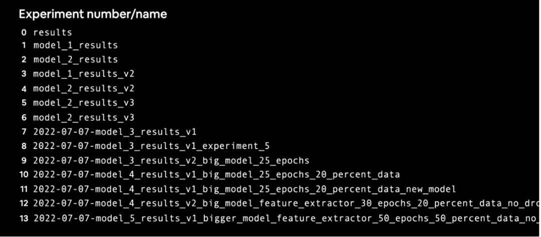
在构建了一些模型并跟踪其结果后,您会开始注意到它会以多快的速度失控。
Different ways to track machine learning experiments
下面是跟踪机器学习实验的一些方法。
| Method | Setup | Pros | Cons | Cost |
| Python字典, CSV, print | 无 | 简单使用,直接在原始的Python中使用 | 难以追踪大量的实验 | Free |
| TensorBoard | 安装 tensorboard | 对PyTorch的扩展,广泛认可和使用,易于扩展。 | 用户体验不如其他选项好。 | Free |
| Weights & Biases Experiment Tracking | 安装 wandb, 注册 | 令人难以置信的用户体验,公开实验,跟踪几乎所有内容。 | 需要 PyTorch 之外的外部资源。 | Free for personal use |
| MLFlow | 安装 mlflow并开始追踪 | 完全开源的 MLOps 生命周期管理,许多集成。 | 设置远程跟踪服务器比其他服务更难。 | Free |
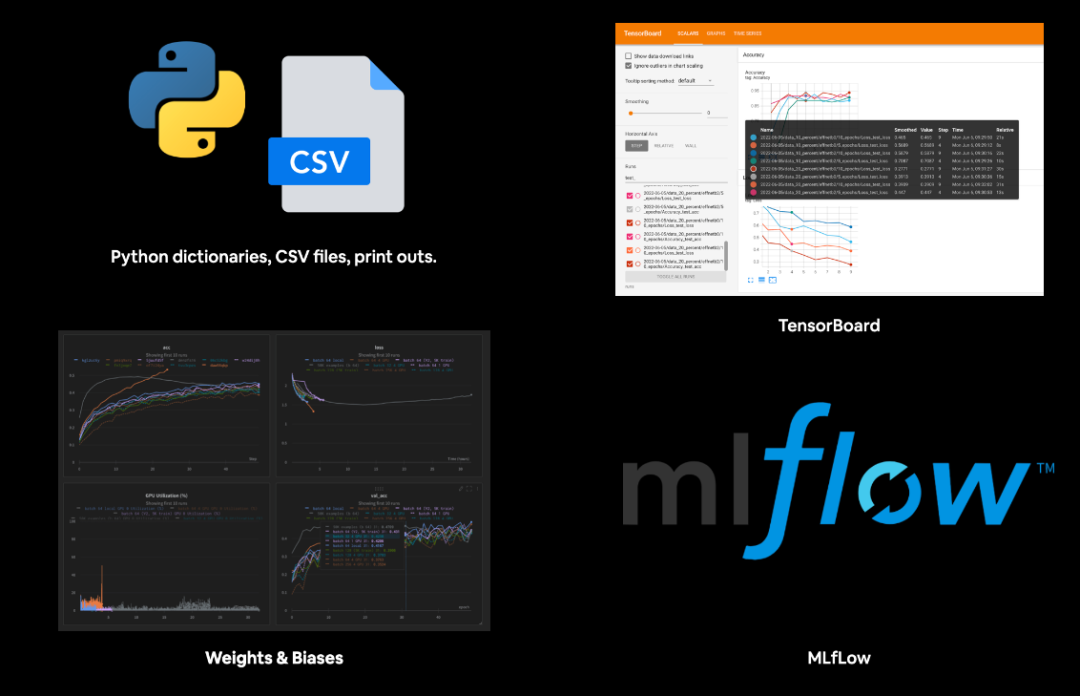
您可以使用各种地点和技术来跟踪您的机器学习实验。 注意: 还有其他各种类似于权重和偏差的选项以及类似于 MLflow 的开源选项,但为简洁起见,我将它们排除在外。您可以通过搜索“机器学习实验跟踪”找到更多信息。
What we're going to cover
我们将使用不同级别的数据、模型大小和训练时间运行几个不同的建模实验,以尝试和改进 FoodVision Mini。由于TensorBoard
与 PyTorch 的紧密集成和广泛使用,这个 notebook 专注于使用 TensorBoard
来跟踪我们的实验。但是,我们将要介绍的原则在所有其他用于实验跟踪的工具中都是相似的。
| Topic | Contents |
| 0. Getting setup | 我们在过去的几节中编写了一些有用的代码,让我们下载它并确保我们可以再次使用它。 |
| 1. Get data | 让我们获取我们一直用来尝试改进 FoodVision Mini 模型结果的比萨饼、牛排和寿司图像分类数据集。 |
| 2. Create Datasets and DataLoaders | 使用05中写的 data_setup.py创建DataLoader |
| 3. Get and customise a pretrained model | 类似06,下载 torchvision.models的预训练模型并做修改 |
| 4. Train model amd track results | 让我们看看使用 TensorBoard 训练和跟踪单个模型的训练结果是什么感觉。 |
| 5. View our model's results in TensorBoard | 之前我们使用辅助函数可视化模型的损失曲线,现在让我们看看它们在 TensorBoard 中的样子。 |
| 6. Creating a helper function to track experiments | 如果我们要坚持机器学习从业者的格言实验、实验、实验!,我们最好创建一个函数来帮助我们保存我们的建模实验结果。 |
| 7. Setting up a series of modelling experiments | 与其一个接一个地运行实验,不如我们编写一些代码来一次运行多个实验,使用不同的模型、不同的数据量和不同的训练时间。 |
| 8. View modelling experiments in TensorBoard | 在这个阶段,我们将一次性运行八个建模实验,需要跟踪一些,让我们看看它们在 TensorBoard 中的结果。 |
| 9. Load in the best model and make predictions with it | 实验跟踪的重点是找出哪个模型表现最好,让我们加载表现最好的模型并用它做出一些预测以可视化、可视化、可视化!。 |
0. Getting setup
让我们首先下载本节所需的所有模块。为了节省我们编写额外代码的时间,我们将利用我们在 05. PyTorch 走向模块化。
具体来说,我们将从 pytorch-deep-learning
存储库下载 going_modular
目录。如果 torchinfo
包不可用,我们还将安装它。torchinfo
将帮助我们稍后为我们的模型提供摘要。
# For this notebook to run with updated APIs, we need torch 1.12+ and torchvision 0.13+
try:
    import torch
    import torchvision
    assert int(torch.__version__.split(".")[1]) >= 12, "torch version should be 1.12+"
    assert int(torchvision.__version__.split(".")[1]) >= 13, "torchvision version should be 0.13+"
    print(f"torch version: {torch.__version__}")
    print(f"torchvision version: {torchvision.__version__}")
except:
    print(f"[INFO] torch/torchvision versions not as required, installing nightly versions.")
    !pip3 install -U torch torchvision torchaudio --extra-index-url https://download.pytorch.org/whl/cu113
    import torch
    import torchvision
    print(f"torch version: {torch.__version__}")
    print(f"torchvision version: {torchvision.__version__}")
# Continue with regular imports
import matplotlib.pyplot as plt
import torch
import torchvision

from torch import nn
from torchvision import transforms

# Try to get torchinfo, install it if it doesn't work
try:
    from torchinfo import summary
except:
    print("[INFO] Couldn't find torchinfo... installing it.")
    !pip install -q torchinfo
    from torchinfo import summary

# Try to import the going_modular directory, download it from GitHub if it doesn't work
try:
    from going_modular.going_modular import data_setup, engine
except:
    # Get the going_modular scripts
    print("[INFO] Couldn't find going_modular scripts... downloading them from GitHub.")
    !git clone https://github.com/mrdbourke/pytorch-deep-learning
    !mv pytorch-deep-learning/going_modular .
    !rm -rf pytorch-deep-learning
    from going_modular.going_modular import data_setup, engine
device = "cuda" if torch.cuda.is_available() else "cpu"
device
'cuda'
Create a helper function to set seeds
由于我们在前面的部分中设置了一大堆随机种子,我们为什么不用函数实现呢?让我们创建一个设置随机种子的函数set_seeds()
。
# Set seeds
def set_seeds(seed: int=42):
    """Sets random sets for torch operations.

    Args:
        seed (int, optional): Random seed to set. Defaults to 42.
    """
    # Set the seed for general torch operations
    torch.manual_seed(seed)
    # Set the seed for CUDA torch operations (ones that happen on the GPU)
    torch.cuda.manual_seed(seed)
1. Get data
与往常一样,在我们运行机器学习实验之前,我们需要一个数据集。我们将继续努力改进我们在 FoodVision Mini 上获得的结果。
让我们下载准备好的数据集。
import os
import zipfile

from pathlib import Path

import requests

def download_data(source: str,
                  destination: str,
                  remove_source: bool = True) -> Path:
    """Downloads a zipped dataset from source and unzips to destination.

    Args:
        source (str): A link to a zipped file containing data.
        destination (str): A target directory to unzip data to.
        remove_source (bool): Whether to remove the source after downloading and extracting.

    Returns:
        pathlib.Path to downloaded data.

    Example usage:
        download_data(source="https://github.com/mrdbourke/pytorch-deep-learning/raw/main/data/pizza_steak_sushi.zip",
                      destination="pizza_steak_sushi")
    """
    # Setup path to data folder
    data_path = Path("data/")
    image_path = data_path / destination

    # If the image folder doesn't exist, download it and prepare it...
    if image_path.is_dir():
        print(f"[INFO] {image_path} directory exists, skipping download.")
    else:
        print(f"[INFO] Did not find {image_path} directory, creating one...")
        image_path.mkdir(parents=True, exist_ok=True)

        # Download pizza, steak, sushi data
        target_file = Path(source).name
        with open(data_path / target_file, "wb") as f:
            request = requests.get(source)
            print(f"[INFO] Downloading {target_file} from {source}...")
            f.write(request.content)

        # Unzip pizza, steak, sushi data
        with zipfile.ZipFile(data_path / target_file, "r") as zip_ref:
            print(f"[INFO] Unzipping {target_file} data...")
            zip_ref.extractall(image_path)

        # Remove .zip file
        if remove_source:
            os.remove(data_path / target_file)

    return image_path

image_path = download_data(source="https://github.com/mrdbourke/pytorch-deep-learning/raw/main/data/pizza_steak_sushi.zip",
                           destination="pizza_steak_sushi")
image_path
[INFO] data\pizza_steak_sushi directory exists, skipping download.
WindowsPath('data/pizza_steak_sushi')
2. Create Datasets and DataLoaders
现在我们有了一些数据,让我们把它变成 PyTorch DataLoaders。
我们可以使用我们在 05. PyTorch 模块化第 2 部分。
由于我们将使用迁移学习和来自 torchvision.models
的专门预训练模型,我们将创建一个转换来正确准备我们的图像.
要将我们的图像转换为张量,我们可以使用:
1. 使用
torchvision.transforms
手动创建变换。2. 使用
torchvision.models.MODEL_NAME.MODEL_WEIGHTS.DEFAULT.transforms()
自动创建转换。
我们在 06. PyTorch 迁移学习第 2 部分有过类似的操作。
让我们首先看一个手动创建“torchvision.transforms”管道的示例(以这种方式创建转换管道可以提供最多的自定义,但如果转换与预训练模型不匹配,可能会导致性能下降)。
我们需要确定的主要手动转换是我们所有的图像都以 ImageNet 格式标准化(这是因为预训练的 torchvision.models
都是在 ImageNet 上预训练的。
我们可以这样做:
normalize = transforms.Normalize(mean=[0.485, 0.456, 0.406],
                                 std=[0.229, 0.224, 0.225])
2.1 Create DataLoaders using manually created transforms
# Setup directories
train_dir = image_path / "train"
test_dir = image_path / "test"

# Setup ImageNet normalization levels (turns all images into similar distribution as ImageNet)
normalize = transforms.Normalize(mean=[0.485, 0.456, 0.406],
                                 std=[0.229, 0.224, 0.225])

# Create transform pipeline manually
manual_transforms = transforms.Compose([
    transforms.Resize((224, 224)),
    transforms.ToTensor(),
    normalize
])
print(f"Manually created transforms: {manual_transforms}")

# Create data loaders
train_dataloader, test_dataloader, class_names = data_setup.create_dataloaders(
    train_dir=train_dir,
    test_dir=test_dir,
    transform=manual_transforms, # use manually created transforms
    batch_size=32
)

train_dataloader, test_dataloader, class_names
2.2 Create DataLoaders using automatically created transforms
现在让我们看看自动转换是什么样的。我们可以通过首先实例化一组我们想要使用的预训练权重(例如 weights = torchvision.models.EfficientNet_B0_Weights.DEFAULT
)并在其上调用 transforms()
方法来做到这一点。
# Setup dirs
train_dir = image_path / "train"
test_dir = image_path / "test"

# Setup pretrained weights (plenty of these available in torchvision.models)
weights = torchvision.models.EfficientNet_B0_Weights.DEFAULT

# Get transforms from weights (these are the transforms that were used to obtain the weights)
automatic_transforms = weights.transforms()
print(f"Automatically created transforms: {automatic_transforms}")

# Create data loaders
train_dataloader, test_dataloader, class_names = data_setup.create_dataloaders(
    train_dir=train_dir,
    test_dir=test_dir,
    transform=automatic_transforms, # use automatic created transforms
    batch_size=32
)

train_dataloader, test_dataloader, class_names
3. Getting a pretrained model, freezing the base layers and changing the classifier head
在我们运行和跟踪多个建模实验之前,让我们看看运行和跟踪单个实验是什么感觉。
既然我们的数据已经准备好了,接下来我们需要的是一个模型。让我们下载torchvision.models.efficientnet_b0()
模型的预训练权重,并准备好与我们自己的数据一起使用。
# Note: This is how a pretrained model would be created in torchvision > 0.13, it will be deprecated in future versions.
# model = torchvision.models.efficientnet_b0(pretrained=True).to(device) # OLD

# Download the pretrained weights for EfficientNet_B0
weights = torchvision.models.EfficientNet_B0_Weights.DEFAULT # NEW in torchvision 0.13, "DEFAULT" means "best weights available"

# Setup the model with the pretrained weights and send it to the target device
model = torchvision.models.efficientnet_b0(weights=weights).to(device)
现在我们有了一个预训练的模型,让我们对模型做一些调整。我们将冻结模型的基础层(我们将使用它们从输入图像中提取特征),我们将更改分类器头(输出层)以适应我们正在使用的类的数量 (我们有 3 类:比萨、牛排、寿司)。
# Freeze all base layers by setting requires_grad attribute to False
for param in model.features.parameters():
    param.requires_grad = False

# Since we're creating a new layer with random weights (torch.nn.Linear),
# let's set the seeds
set_seeds()

# Update the classifier head to suit our problem
model.classifier = torch.nn.Sequential(
    nn.Dropout(p=0.2, inplace=True),
    nn.Linear(in_features=1280,
              out_features=len(class_names),
              bias=True).to(device))
可以用 torchinfo.summary()
来查看模型结构。
from torchinfo import summary

# # Get a summary of the model (uncomment for full output)
# summary(model,
#         input_size=(32, 3, 224, 224), # make sure this is "input_size", not "input_shape" (batch_size, color_channels, height, width)
#         verbose=0,
#         col_names=["input_size", "output_size", "num_params", "trainable"],
#         col_width=20,
#         row_settings=["var_names"]
# )

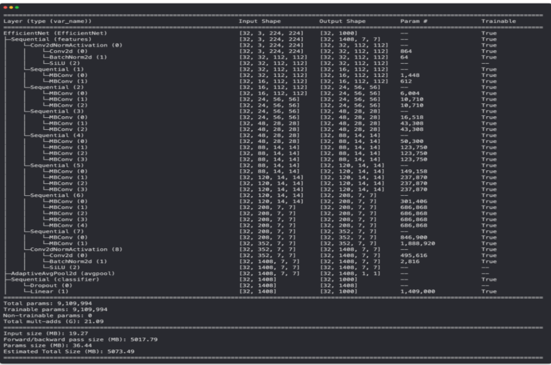
使用我们的特征提取器 EffNetB0 模型输出torchinfo.summary()
,注意基础层是如何被冻结的(不可训练的),输出层是如何根据我们自己的问题定制的。
4. Train model and track results
让我们准备好通过创建损失函数和优化器来训练它。由于我们正在处理多个类,我们将使用 torch.nn.CrossEntropyLoss()
作为loss。我们将坚持使用 torch.optim.Adam()
,优化器的学习率为 0.001
。
# Define loss and optimizer
loss_fn = nn.CrossEntropyLoss()
optimizer = torch.optim.Adam(model.parameters(), lr=0.001)
Adjust train()
function to track results with SummaryWriter()
现在让我们添加最后一块来跟踪我们的实验。以前,我们使用多个 Python 字典(每个模型一个)来跟踪我们的建模实验。但是你可以想象,如果我们只进行几个实验,这可能会失控。不用担心,还有更好的选择!我们可以使用 PyTorch 的 torch.utils.tensorboard.SummaryWriter()
类将模型训练进度的各个部分保存到文件中。
默认情况下,SummaryWriter()
类将有关我们模型的各种信息保存到由 log_dir
参数设置的文件中。 log_dir
的默认位置在 runs/CURRENT_DATETIME_HOSTNAME
下,其中 HOSTNAME
是您计算机的名称。您可以更改log_dir
保存信息到其它位置。
SummaryWriter()
的输出以 TensorBoard 格式 保存。TensorBoard 是 TensorFlow 深度学习库的一部分,是可视化模型不同部分的绝佳方式。
为了开始跟踪我们的建模实验,让我们创建一个默认的SummaryWriter()
实例。
from torch.utils.tensorboard import SummaryWriter

# Create a writer with all default settings
writer = SummaryWriter()
现在要使用 writer,我们可以编写一个新的训练循环,或者调整我们在 05. PyTorch Going Modular 第 4 节。
让我们采取后一种选择。我们将从 engine.py
获取 train()
函数并进行调整它使用writer
。
具体来说,我们将为train()
函数添加记录模型的训练和测试损失和准确度值的能力。可以使用 writer.add_scalars(main_tag, tag_scalar_dict)
来做到这一点,其中:
•
main_tag
(string) - 被跟踪的标量的名称(例如“Accuracy”)•
tag_scalar_dict
(dict) - 被跟踪值的字典(例如{"train_loss": 0.3454}
)•
注意: 该方法被称为
add_scalars()
因为我们的损失和准确率值通常是标量(单值)。
一旦我们完成跟踪值,我们将调用 writer.close()
来告诉 writer
停止寻找要跟踪的值。
要开始修改 train()
,我们还将从 engine.py
导入 train_step()
和 test_step()
。
注意: 您几乎可以在代码中的任何位置跟踪有关模型的信息。但是经常会在模型训练时(在训练/测试循环内)跟踪实验。
torch.utils.tensorboard.SummaryWriter()
类也有许多不同的方法来跟踪关于你的模型/数据的不同事物,例如add_graph()
跟踪模型的计算图。更多选项,查看SummaryWriter()
文档。
from typing import Dict, List
from tqdm.auto import tqdm

from going_modular.going_modular.engine import train_step, test_step

# Import train() function from:
# https://github.com/mrdbourke/pytorch-deep-learning/blob/main/going_modular/going_modular/engine.py
def train(model: torch.nn.Module,
          train_dataloader: torch.utils.data.DataLoader,
          test_dataloader: torch.utils.data.DataLoader,
          optimizer: torch.optim.Optimizer,
          loss_fn: torch.nn.Module,
          epochs: int,
          device: torch.device) -> Dict[str, List]:

    # Create empty results dictionary
    results = {"train_loss": [],
               "train_acc": [],
               "test_loss": [],
               "test_acc": []
    }

    # Loop through training and testing steps for a number of epochs
    for epoch in tqdm(range(epochs)):
        train_loss, train_acc = train_step(model=model,
                                           dataloader=train_dataloader,
                                           loss_fn=loss_fn,
                                           optimizer=optimizer,
                                           device=device)
        test_loss, test_acc = test_step(model=model,
                                        dataloader=test_dataloader,
                                        loss_fn=loss_fn,
                                        device=device)

        # Print out what's happening
        print(
          f"Epoch: {epoch+1} | "
          f"train_loss: {train_loss:.4f} | "
          f"train_acc: {train_acc:.4f} | "
          f"test_loss: {test_loss:.4f} | "
          f"test_acc: {test_acc:.4f}"
        )

        # Update results dictionary
        results["train_loss"].append(train_loss)
        results["train_acc"].append(train_acc)
        results["test_loss"].append(test_loss)
        results["test_acc"].append(test_acc)

        ### New: Experiment tracking ###
        # Add loss results to SummaryWriter
        writer.add_scalars(main_tag="Loss",
                           tag_scalar_dict={"train_loss": train_loss,
                                            "test_loss": test_loss},
                           global_step=epoch)

        # Add accuracy results to SummaryWriter
        writer.add_scalars(main_tag="Accuracy",
                           tag_scalar_dict={"train_acc": train_acc,
                                            "test_acc": test_acc},
                           global_step=epoch)

        # Track the PyTorch model architecture
        writer.add_graph(model=model,
                         # Pass in an example input
                         input_to_model=torch.randn(32, 3, 224, 224).to(device))

    # Close the writer
    writer.close()

    ### End new ###

    # Return the filled results at the end of the epochs
    return results
我们的 train()
函数现在使用 SummaryWriter()
实例来跟踪我们模型的结果。我们尝试 5 个 epoch 看看效果。
# Train model
# Note: Not using engine.train() since the original script isn't updated to use writer
set_seeds()
results = train(model=model,
                train_dataloader=train_dataloader,
                test_dataloader=test_dataloader,
                optimizer=optimizer,
                loss_fn=loss_fn,
                epochs=5,
                device=device)
  0%|          | 0/5 [00:00<?, ?it/s]


Epoch: 1 | train_loss: 1.0948 | train_acc: 0.3984 | test_loss: 0.9034 | test_acc: 0.6411
Epoch: 2 | train_loss: 0.9005 | train_acc: 0.6445 | test_loss: 0.7874 | test_acc: 0.8561
Epoch: 3 | train_loss: 0.8115 | train_acc: 0.7500 | test_loss: 0.6749 | test_acc: 0.8759
Epoch: 4 | train_loss: 0.6853 | train_acc: 0.7383 | test_loss: 0.6704 | test_acc: 0.8352
Epoch: 5 | train_loss: 0.7091 | train_acc: 0.7383 | test_loss: 0.6768 | test_acc: 0.8040
运行上面的单元格,我们得到与 06. PyTorch 迁移学习第 4 部分:训练模型类似的结果,不同之处在于 writer
实例创建了一个 runs/
目录存储模型的结果。
例如,保存位置可能如下所示:
runs/Jun21_00-46-03_daniels_macbook_pro
默认格式是runs/CURRENT_DATETIME_HOSTNAME
。
我们将在一秒钟内检查这些,但作为提醒,我们之前在字典中跟踪我们模型的结果。
# Check out the model results
results
{'train_loss': [1.09475726634264,
  0.9005270600318909,
  0.8115105107426643,
  0.6853345558047295,
  0.7091127447783947],
 'train_acc': [0.3984375, 0.64453125, 0.75, 0.73828125, 0.73828125],
 'test_loss': [0.9034053285916647,
  0.7874306440353394,
  0.6748601198196411,
  0.6704476873079935,
  0.6768251856168112],
 'test_acc': [0.6410984848484849,
  0.8560606060606061,
  0.8759469696969697,
  0.8352272727272728,
  0.8039772727272728]}
嗯,我们可以把它格式化成一个很好的图,但你能想象一下跟踪一堆这些字典吗?
一定有更好的方法...
5. View our model's results in TensorBoard
SummaryWriter()
类默认将模型的结果以 TensorBoard 格式存储在名为 runs/
的目录中。TensorBoard 是由 TensorFlow 团队创建的可视化程序,用于查看和检查有关模型和数据的信息。您可以通过多种方式查看 TensorBoard:
| Code environment | How to view TensorBoard | Resource |
| VS Code (notebooks or Python scripts) | Press SHIFT + CMD + Pto open the Command Palette and search for the command "Python: Launch TensorBoard". | VS Code Guide on TensorBoard and PyTorch |
| Jupyter and Colab Notebooks | Make sure TensorBoard is installed, load it with %load_ext tensorboardand then view your results with %tensorboard --logdir DIR_WITH_LOGS. | torch.utils.tensorboardand Get started with TensorBoard |
您还可以将您的实验上传到 tensorboard.dev 与他人公开分享。
在 Google Colab 或 Jupyter Notebook 中运行以下代码将启动交互式 TensorBoard 会话以查看 runs/
目录中的 TensorBoard 文件.
# Example code to run in Jupyter or Google Colab Notebook (uncomment to try it out)
%load_ext tensorboard
%tensorboard --logdir runs
如果一切正常,您应该会看到如下内容:
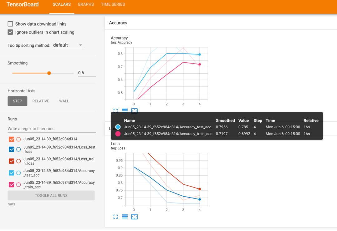
在 TensorBoard 中查看单个建模实验的准确度和损失结果。
注意:有关在笔记本或其他位置运行 TensorBoard 的更多信息,请参阅以下内容:
• TensorFlow 在笔记本中使用 TensorBoard 指南
• 开始使用 TensorBoard.dev(有助于将 TensorBoard 日志上传到可共享链接)
6. Create a helper function to build SummaryWriter()
instances
SummaryWriter()
类将各种信息记录到由 log_dir
参数指定的目录中。我们如何创建一个辅助函数来为每个实验创建一个自定义目录?
本质上,每个实验都有自己的日志目录。例如,假设我们要跟踪以下内容:
• 实验日期/时间戳 - 实验何时进行?
• 实验名称 - 有什么我们想为实验命名的东西吗?
• model名称 - 使用什么model?
• 额外 - 是否应该跟踪其他任何内容?
您可以在这里跟踪几乎所有内容,并随心所欲地发挥创意,但这些应该足以开始。让我们创建一个名为 create_writer()
的辅助函数,它生成一个 SummaryWriter()
实例跟踪到自定义 log_dir
。
理想情况下,我们希望 log_dir
类似于: runs/YYYY-MM-DD/experiment_name/model_name/extra
其中 YYYY-MM-DD
是实验运行的日期(如果您愿意,也可以添加时间)。
def create_writer(experiment_name: str,
                  model_name: str,
                  extra: str=None) -> torch.utils.tensorboard.writer.SummaryWriter():
    """Creates a torch.utils.tensorboard.writer.SummaryWriter() instance saving to a specific log_dir.

    log_dir is a combination of runs/timestamp/experiment_name/model_name/extra.

    Where timestamp is the current date in YYYY-MM-DD format.

    Args:
        experiment_name (str): Name of experiment.
        model_name (str): Name of model.
        extra (str, optional): Anything extra to add to the directory. Defaults to None.

    Returns:
        torch.utils.tensorboard.writer.SummaryWriter(): Instance of a writer saving to log_dir.

    Example usage:
        # Create a writer saving to "runs/2022-06-04/data_10_percent/effnetb2/5_epochs/"
        writer = create_writer(experiment_name="data_10_percent",
                               model_name="effnetb2",
                               extra="5_epochs")
        # The above is the same as:
        writer = SummaryWriter(log_dir="runs/2022-06-04/data_10_percent/effnetb2/5_epochs/")
    """
    from datetime import datetime
    import os

    # Get timestamp of current date (all experiments on certain day live in same folder)
    timestamp = datetime.now().strftime("%Y-%m-%d") # returns current date in YYYY-MM-DD format

    if extra:
        # Create log directory path
        log_dir = os.path.join("runs", timestamp, experiment_name, model_name, extra)
    else:
        log_dir = os.path.join("runs", timestamp, experiment_name, model_name)

    print(f"[INFO] Created SummaryWriter, saving to: {log_dir}...")
    return SummaryWriter(log_dir=log_dir)
让我们试一试:
# Create an example writer
example_writer = create_writer(experiment_name="data_10_percent",
                               model_name="effnetb0",
                               extra="5_epochs")
[INFO] Created SummaryWriter, saving to: runs\2022-09-17\data_10_percent\effnetb0\5_epochs...
看起来不错,现在我们有了记录和追溯各种实验的方法。
6.1 Update the train()
function to include a writer
parameter
我们的 create_writer()
函数效果很好。我们如何让我们的 train()
函数能够接收 writer
参数,以便我们在每次调用 train()
时主动更新我们正在使用的 SummaryWriter()
实例。
例如,假设我们正在运行一系列实验,为多个不同的模型多次调用 train()
,如果每个实验使用不同的 writer
会很好。
每个实验一个 writer
= 每个实验一个日志目录。为了调整 train()
函数,我们将向函数添加 writer
参数,然后我们将添加一些代码来查看是否有 writer
,如果有,我们将在那里跟踪我们的信息。
from typing import Dict, List
from tqdm.auto import tqdm

# Add writer parameter to train()
def train(model: torch.nn.Module,
          train_dataloader: torch.utils.data.DataLoader,
          test_dataloader: torch.utils.data.DataLoader,
          optimizer: torch.optim.Optimizer,
          loss_fn: torch.nn.Module,
          epochs: int,
          device: torch.device,
          writer: torch.utils.tensorboard.writer.SummaryWriter # new parameter to take in a writer
          ) -> Dict[str, List]:
    # Create empty results dictionary
    results = {"train_loss": [],
               "train_acc": [],
               "test_loss": [],
               "test_acc": []
    }

    # Loop through training and testing steps for a number of epochs
    for epoch in tqdm(range(epochs)):
        train_loss, train_acc = train_step(model=model,
                                          dataloader=train_dataloader,
                                          loss_fn=loss_fn,
                                          optimizer=optimizer,
                                          device=device)
        test_loss, test_acc = test_step(model=model,
          dataloader=test_dataloader,
          loss_fn=loss_fn,
          device=device)

        # Print out what's happening
        print(
          f"Epoch: {epoch+1} | "
          f"train_loss: {train_loss:.4f} | "
          f"train_acc: {train_acc:.4f} | "
          f"test_loss: {test_loss:.4f} | "
          f"test_acc: {test_acc:.4f}"
        )

        # Update results dictionary
        results["train_loss"].append(train_loss)
        results["train_acc"].append(train_acc)
        results["test_loss"].append(test_loss)
        results["test_acc"].append(test_acc)


        ### New: Use the writer parameter to track experiments ###
        # See if there's a writer, if so, log to it
        if writer:
            # Add results to SummaryWriter
            writer.add_scalars(main_tag="Loss",
                               tag_scalar_dict={"train_loss": train_loss,
                                                "test_loss": test_loss},
                               global_step=epoch)
            writer.add_scalars(main_tag="Accuracy",
                               tag_scalar_dict={"train_acc": train_acc,
                                                "test_acc": test_acc},
                               global_step=epoch)

            # Close the writer
            writer.close()
        else:
            pass
    ### End new ###

    # Return the filled results at the end of the epochs
    return results
7. Setting up a series of modelling experiments
以前我们一直在进行各种实验,并一一检查结果。但是,如果我们可以运行多个实验,然后一起检查结果呢?
7.1 What kind of experiments should you run?
多数时候并不能确定哪些参数对实验重要。每个超参数都代表不同实验的起点:
• 更改 epochs 的数量。
• 更改层/隐藏单元的数量。
• 更改数据的数量。
• 更改学习率。
• 尝试不同类型的数据增强。
• 选择不同的模型架构。
通过练习和运行许多不同的实验,您将开始建立对可能对您的模型有什么帮助的直觉。总的来说,鉴于 The Bitter Lesson(我现在已经提到过两次,因为它是 AI 世界中的一篇重要文章), 通常,您的模型越大(可学习的参数越多)和拥有的数据越多(学习机会越多),性能就越好。
但是,当您第一次处理机器学习问题时:从小处着手,如果可行,请扩大规模。您的第一批实验的运行时间不应超过几秒到几分钟。实验越快,你就能越快找出不起作用的东西,反过来,你就能越快找出起作用的东西。
7.2 What experiments are we going to run?
我们的目标是改进为 FoodVision Mini 提供动力的模型,但不会变得太大。从本质上讲,我们理想的模型实现了高水平的测试集准确度(90% 以上),但训练/执行推理(做出预测)不需要太长时间。
我们有很多选择,但我们如何保持简单?让我们尝试以下组合:
1. 不同数量的数据(披萨、牛排、寿司的 10% vs. 20%)
2. 不同的模型(
torchvision.models.efficientnet_b0
与torchvision. models.efficientnet_b2
)3. 不同的训练时间(5 epochs vs. 10 epochs)
组合后我们可以得到8种实验(2^3)。在每次实验中,我们都会慢慢增加数据量、模型大小和训练时间。到最后,与实验 1 相比,实验 8 将使用双倍的数据、双倍的模型大小和双倍的训练时间。
注意: 我想明确一点,您可以运行的实验数量确实没有限制。我们在这里设计的只是选项的一小部分。但是,您无法测试所有内容,因此最好先尝试一些事情,然后再遵循最有效的事情。
提醒一下,我们使用的数据集是 Food101 数据集 的子集 (3 类,披萨、牛排、suhsi,而不是 101)和 10% 和 20% 的图像而不是 100%。如果我们的实验成功,我们可以开始在更多数据上运行更多(尽管这需要更长的计算时间)。您可以通过
04_custom_data_creation.ipynb
笔记本查看数据集是如何创建的。
7.3 Download different datasets
在开始前,我们要确保数据集准备好了。我们需要2种数据集:
1. A training set with 10% of the data of Food101 pizza, steak, sushi images.
2. A training set with 20% of the data of Food101 pizza, steak, sushi images.
为了保持一致性,所有实验都将使用相同的测试数据集(来自 10% 数据拆分的数据集)。
让我们下载数据集吧。它们在课程相关的GitHub上:
1. Pizza, steak, sushi 10% training data.
2. Pizza, steak, sushi 20% training data.
# Download 10 percent and 20 percent training data (if necessary)
data_10_percent_path = download_data(source="https://github.com/mrdbourke/pytorch-deep-learning/raw/main/data/pizza_steak_sushi.zip",
                                     destination="pizza_steak_sushi")

data_20_percent_path = download_data(source="https://github.com/mrdbourke/pytorch-deep-learning/raw/main/data/pizza_steak_sushi_20_percent.zip",
                                     destination="pizza_steak_sushi_20_percent")
数据下载完成后,继续设置将用于不同实验的数据的文件路径。我们将创建不同的训练目录路径,但我们只需要一个测试目录路径,因为所有实验都将使用相同的测试数据集(来自披萨、牛排、寿司的测试数据集 10%)。
# Setup training directory paths
train_dir_10_percent = data_10_percent_path / "train"
train_dir_20_percent = data_20_percent_path / "train"

# Setup testing directory paths (note: use the same test dataset for both to compare the results)
test_dir = data_10_percent_path / "test"

# Check the directories
print(f"Training directory 10%: {train_dir_10_percent}")
print(f"Training directory 20%: {train_dir_20_percent}")
print(f"Testing directory: {test_dir}")
7.4 Transform Datasets and create DataLoaders
接下来,我们将创建一系列转换来为我们的模型准备图像。为了保持一致,我们将手动创建一个变换(就像我们上面所做的那样)并在所有数据集上使用相同的变换。
转换将:
1. 调整所有图像的大小(我们将从 224、224 开始,但可以更改)。
2. 将它们变成值在 0 和 1 之间的张量。
3. 以某种方式对它们进行归一化,使其分布与 ImageNet 数据集内联(我们这样做是因为我们来自
torchvision.models
的模型已经过预训练 在 ImageNet 上)。
from torchvision import transforms

# Create a transform to normalize data distribution to be inline with ImageNet
normalize = transforms.Normalize(mean=[0.485, 0.456, 0.406], # values per colour channel [red, green, blue]
                                 std=[0.229, 0.224, 0.225]) # values per colour channel [red, green, blue]

# Compose transforms into a pipeline
simple_transform = transforms.Compose([
    transforms.Resize((224, 224)), # 1. Resize the images
    transforms.ToTensor(), # 2. Turn the images into tensors with values between 0 & 1
    normalize # 3. Normalize the images so their distributions match the ImageNet dataset
])
现在让我们使用我们在 05. PyTorch Going Modular 第 2 节写好的DataLoader。
我们将创建批量大小为 32 的 DataLoader。对于我们所有的实验,我们将使用相同的“test_dataloader”(以保持比较一致)。
BATCH_SIZE = 32

# Create 10% training and test DataLoaders
train_dataloader_10_percent, test_dataloader, class_names = data_setup.create_dataloaders(train_dir=train_dir_10_percent,
    test_dir=test_dir,
    transform=simple_transform,
    batch_size=BATCH_SIZE
)

# Create 20% training and test data DataLoders
train_dataloader_20_percent, test_dataloader, class_names = data_setup.create_dataloaders(train_dir=train_dir_20_percent,
    test_dir=test_dir,
    transform=simple_transform,
    batch_size=BATCH_SIZE
)

# Find the number of samples/batches per dataloader (using the same test_dataloader for both experiments)
print(f"Number of batches of size {BATCH_SIZE} in 10 percent training data: {len(train_dataloader_10_percent)}")
print(f"Number of batches of size {BATCH_SIZE} in 20 percent training data: {len(train_dataloader_20_percent)}")
print(f"Number of batches of size {BATCH_SIZE} in testing data: {len(train_dataloader_10_percent)} (all experiments will use the same test set)")
print(f"Number of classes: {len(class_names)}, class names: {class_names}")
7.5 Create feature extractor models
是时候开始构建我们的模型了。我们将创建两个特征提取器模型:
1.
torchvision.models.efficientnet_b0()
预训练主干+自定义分类器头(简称EffNetB0)。2.
torchvision.models.efficientnet_b2()
预训练主干+自定义分类器头(简称EffNetB2)。
为此,我们将冻结基础层(特征层)并更新模型的分类器头(输出层)以适应我们的问题,就像我们在 06. PyTorch 迁移学习第 3.4 节。
我们在上一章中看到 EffNetB0 的分类器头的 in_features
参数是 1280
(主干将输入图像转换为大小为 1280
的特征向量)。
由于 EffNetB2 具有不同数量的层和参数,因此我们需要相应地对其进行调整。
注意: 每当您使用不同的模型时,您首先应该检查的事情之一是输入和输出形状。这样,您将知道如何准备输入数据/更新模型以获得正确的输出形状。
我们可以使用 torchinfo.summary()
并传入 input_size=(32, 3, 224, 224)
找到 EffNetB2 的输入和输出形状 参数((32, 3, 224, 224)
等价于 (batch_size, color_channels, height, width)
,即我们传入一个示例,说明一批数据对我们的模型的影响)。
注意: 许多现代模型可以处理不同大小的输入图像,这要归功于 [
torch.nn.AdaptiveAvgPool2d()
](https://pytorch.org/docs/stable/generated/torch.nn.AdaptiveAvgPool2d .html) 层,该层根据需要自适应地调整给定输入的output_size
。您可以通过将不同大小的输入图像传递给“torchinfo.summary()”或使用该层的您自己的模型来尝试这一点。
为了找到 EffNetB2 最后一层所需的输入形状,让我们:
1. 创建一个
torchvision.models.efficientnet_b2(pretrained=True)
的实例。2. 通过运行
torchinfo.summary()
查看各种输入和输出形状。3. 通过检查 EffNetB2 的分类器部分的
state_dict()
并打印权重矩阵的长度,打印出in_features
的数量。• 注意: 你也可以只检查
effnetb2.classifier
的输出。
import torchvision
from torchinfo import summary

# 1. Create an instance of EffNetB2 with pretrained weights
effnetb2_weights = torchvision.models.EfficientNet_B2_Weights.DEFAULT # "DEFAULT" means best available weights
effnetb2 = torchvision.models.efficientnet_b2(weights=effnetb2_weights)

# # 2. Get a summary of standard EffNetB2 from torchvision.models (uncomment for full output)
# summary(model=effnetb2,
#         input_size=(32, 3, 224, 224), # make sure this is "input_size", not "input_shape"
#         # col_names=["input_size"], # uncomment for smaller output
#         col_names=["input_size", "output_size", "num_params", "trainable"],
#         col_width=20,
#         row_settings=["var_names"]
# )

# 3. Get the number of in_features of the EfficientNetB2 classifier layer
print(f"Number of in_features to final layer of EfficientNetB2: {len(effnetb2.classifier.state_dict()['1.weight'][0])}")
EffNetB2 特征提取器模型的模型摘要,所有层均未冻结(可训练)和 ImageNet 预训练的默认分类器头。
现在我们知道了 EffNetB2 模型所需的“in_features”数量,让我们创建几个辅助函数来设置我们的 EffNetB0 和 EffNetB2 特征提取器模型。
我们希望这些功能:
1. 从
torchvision.models
获取基础模型2. 冻结模型中的基础层(设置
requires_grad=False
)3. 设置随机种子(我们不需要*这样做,但由于我们正在运行一系列实验并使用随机权重初始化一个新层,我们希望每个实验的随机性相似)
4. 更改分类器头(以适应我们的问题)
5. 为模型命名(例如,EffNetB0 的“effnetb0”)
import torchvision
from torch import nn

# Get num out features (one for each class pizza, steak, sushi)
OUT_FEATURES = len(class_names)

# Create an EffNetB0 feature extractor
def create_effnetb0():
    # 1. Get the base mdoel with pretrained weights and send to target device
    weights = torchvision.models.EfficientNet_B0_Weights.DEFAULT
    model = torchvision.models.efficientnet_b0(weights=weights).to(device)

    # 2. Freeze the base model layers
    for param in model.features.parameters():
        param.requires_grad = False

    # 3. Set the seeds
    set_seeds()

    # 4. Change the classifier head
    model.classifier = nn.Sequential(
        nn.Dropout(p=0.2),
        nn.Linear(in_features=1280, out_features=OUT_FEATURES)
    ).to(device)

    # 5. Give the model a name
    model.name = "effnetb0"
    print(f"[INFO] Created new {model.name} model.")
    return model

# Create an EffNetB2 feature extractor
def create_effnetb2():
    # 1. Get the base model with pretrained weights and send to target device
    weights = torchvision.models.EfficientNet_B2_Weights.DEFAULT
    model = torchvision.models.efficientnet_b2(weights=weights).to(device)

    # 2. Freeze the base model layers
    for param in model.features.parameters():
        param.requires_grad = False

    # 3. Set the seeds
    set_seeds()

    # 4. Change the classifier head
    model.classifier = nn.Sequential(
        nn.Dropout(p=0.3),
        nn.Linear(in_features=1408, out_features=OUT_FEATURES)
    ).to(device)

    # 5. Give the model a name
    model.name = "effnetb2"
    print(f"[INFO] Created new {model.name} model.")
    return model
让我们通过创建 EffNetB0 和 EffNetB2 的实例并检查它们的“summary()”来测试它们。
effnetb0 = create_effnetb0()
# Get an output summary of the layers in our EffNetB0 feature extractor model (uncomment to view full output)
# summary(model=effnetb0,
#         input_size=(32, 3, 224, 224), # make sure this is "input_size", not "input_shape"
#         # col_names=["input_size"], # uncomment for smaller output
#         col_names=["input_size", "output_size", "num_params", "trainable"],
#         col_width=20,
#         row_settings=["var_names"]
# )
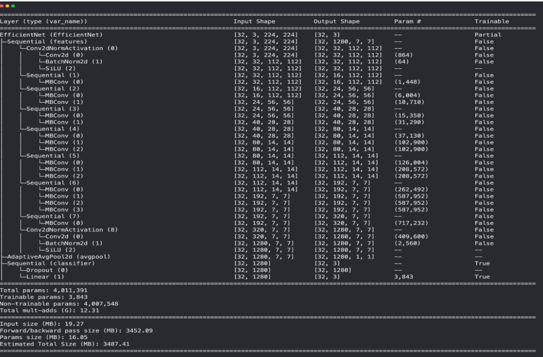
Model summary of EffNetB0 model with base layers frozen (untrainable) and updated classifier head (suited for pizza, steak, sushi image classification).
effnetb2 = create_effnetb2()

# Get an output summary of the layers in our EffNetB2 feature extractor model (uncomment to view full output)
# summary(model=effnetb2,
#         input_size=(32, 3, 224, 224), # make sure this is "input_size", not "input_shape"
#         # col_names=["input_size"], # uncomment for smaller output
#         col_names=["input_size", "output_size", "num_params", "trainable"],
#         col_width=20,
#         row_settings=["var_names"]
# )
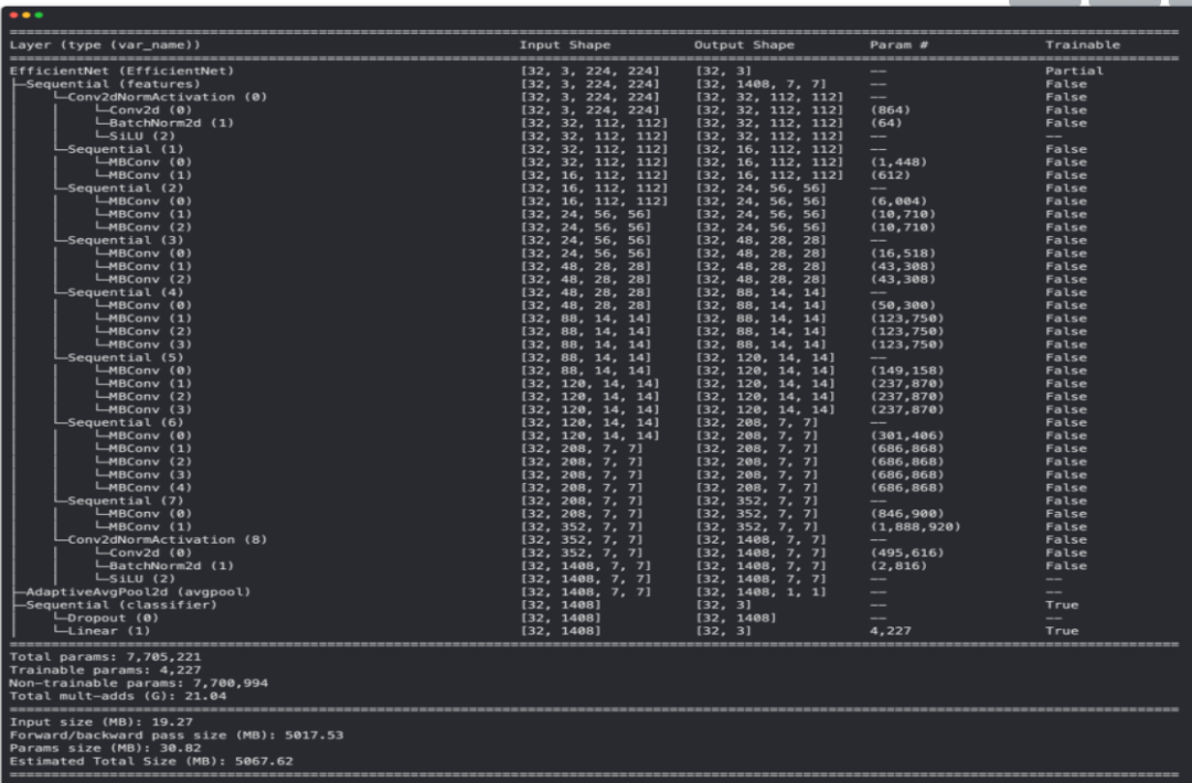
Model summary of EffNetB2 model with base layers frozen (untrainable) and updated classifier head (suited for pizza, steak, sushi image classification).
查看摘要的输出,似乎 EffNetB2 主干的参数数量几乎是 EffNetB0 的两倍。
| Model | Total parameters (before freezing/changing head) | Total parameters (after freezing/changing head) | Total trainable parameters (after freezing/changing head) |
| EfficientNetB0 | 5,288,548 | 4,011,391 | 3,843 |
| EfficientNetB2 | 9,109,994 | 7,705,221 | 4,227 |
这为 EffNetB2 模型的主干提供了更多机会来形成我们的比萨、牛排和寿司数据的表示。但是,每个模型(分类器头)的可训练参数并没有太大的不同。这些额外的参数会带来更好的结果吗?我们将不得不拭目以待......
注意: 本着实验精神,您真的可以尝试几乎任何来自
torchvision.models
的模型,其方式与我们在这里所做的类似。我只选择了 EffNetB0 和 EffNetB2 作为示例。也许您可能想将torchvision.models.convnext_tiny()
或torchvision.models.convnext_small()
之类的东西混在一起。
7.6 Create experiments and set up training code
我们已经准备好数据并准备好模型,是时候进行一些实验了!我们将从创建两个列表和一个字典开始:
1. 我们要测试的 epoch 数量列表(
[5, 10]
)2. 我们要测试的模型列表 (
["effnetb0", "effnetb2"]
)3. 不同训练数据加载器的字典
# 1. Create epochs list
num_epochs = [5, 10]

# 2. Create models list (need to create a new model for each experiment)
models = ["effnetb0", "effnetb2"]

# 3. Create dataloaders dictionary for various dataloaders
train_dataloaders = {"data_10_percent": train_dataloader_10_percent,
                     "data_20_percent": train_dataloader_20_percent}
现在我们可以编写代码来遍历每个不同的选项并尝试每个不同的组合。我们还将在每个实验结束时保存模型,以便稍后我们可以加载回最佳模型并使用它进行预测。
具体来说,让我们通过以下步骤:
1. 设置随机种子(因此我们的实验结果是可重复的,在实践中,您可以在大约 3 个不同的种子上运行相同的实验并对结果进行平均)。
2. 跟踪不同的实验编号(这主要是为了漂亮的打印输出)。
3. 循环遍历每个不同训练 DataLoader 的
train_dataloaders
字典项。4. 循环遍历纪元数列表。
5. 循环浏览不同型号名称的列表。
6. 为当前运行的实验创建信息打印输出(这样我们就知道发生了什么)。
7. 检查哪个模型是目标模型并创建一个新的 EffNetB0 或 EffNetB2 实例(我们每次实验都创建一个新的模型实例,因此所有模型都从相同的角度开始)。
8. 为每个新实验创建一个新的损失函数 (
torch.nn.CrossEntropyLoss()
) 和优化器 (torch.optim.Adam(params=model.parameters(), lr=0.001)
)。9. 使用修改后的
train()
函数训练模型,将适当的细节传递给writer
参数。10. 使用适当的文件名将训练好的模型保存到来自
utils.py
.
我们还可以使用 %%time
魔法来查看我们所有的实验在单个 Jupyter/Google Colab 单元中总共需要多长时间。
我们开始做吧!
%%time
from going_modular.going_modular.utils import save_model

# 1. Set the random seeds
set_seeds(seed=42)

# 2. Keep track of experiment numbers
experiment_number = 0

# 3. Loop through each DataLoader
for dataloader_name, train_dataloader in train_dataloaders.items():

    # 4. Loop through each number of epochs
    for epochs in num_epochs:

        # 5. Loop through each model name and create a new model based on the name
        for model_name in models:

            # 6. Create information print outs
            experiment_number += 1
            print(f"[INFO] Experiment number: {experiment_number}")
            print(f"[INFO] Model: {model_name}")
            print(f"[INFO] DataLoader: {dataloader_name}")
            print(f"[INFO] Number of epochs: {epochs}")

            # 7. Select the model
            if model_name == "effnetb0":
                model = create_effnetb0() # creates a new model each time (important because we want each experiment to start from scratch)
            else:
                model = create_effnetb2() # creates a new model each time (important because we want each experiment to start from scratch)

            # 8. Create a new loss and optimizer for every model
            loss_fn = nn.CrossEntropyLoss()
            optimizer = torch.optim.Adam(params=model.parameters(), lr=0.001)

            # 9. Train target model with target dataloaders and track experiments
            train(model=model,
                  train_dataloader=train_dataloader,
                  test_dataloader=test_dataloader,
                  optimizer=optimizer,
                  loss_fn=loss_fn,
                  epochs=epochs,
                  device=device,
                  writer=create_writer(experiment_name=dataloader_name,
                                       model_name=model_name,
                                       extra=f"{epochs}_epochs"))

            # 10. Save the model to file so we can get back the best model
            save_filepath = f"07_{model_name}_{dataloader_name}_{epochs}_epochs.pth"
            save_model(model=model,
                       target_dir="models",
                       model_name=save_filepath)
            print("-"*50 + "\n")
8. View experiments in TensorBoard
在TensorBoard 中查看结果如何?
# Viewing TensorBoard in Jupyter and Google Colab Notebooks (uncomment to view full TensorBoard instance)
%reload_ext tensorboard
%tensorboard --logdir runs
Reusing TensorBoard on port 6006 (pid 15764), started 1:49:35 ago. (Use '!kill 15764' to kill it.)
运行上面的单元格,我们应该得到类似于以下的输出。

在 TensorBoard 中可视化不同建模实验的测试损失值,可以看到 EffNetB2 模型训练了 10 个 epoch 并使用 20% 的数据实现了最低损失。这符合实验的总体趋势:更多的数据、更大的模型和更长的训练时间通常更好。
您还可以将您的 TensorBoard 实验结果上传到 tensorboard.dev 以免费公开托管它们。
例如,运行类似于以下的代码:
# # Upload the results to TensorBoard.dev (uncomment to try it out)
# !tensorboard dev upload --logdir runs \
#     --name "07. PyTorch Experiment Tracking: FoodVision Mini model results" \
#     --description "Comparing results of different model size, training data amount and training time."
注意: 请注意,您上传到 tensorboard.dev 的任何内容都是公开的,任何人都可以查看。因此,如果您确实上传了您的实验,请注意它们不包含敏感信息。
9. Load in the best model and make predictions with it
查看我们八个实验的 TensorBoard 日志,似乎第 8 个实验取得了最好的整体结果(最高的测试准确度,第二低的测试损失)。
这是使用的实验:
• EffNetB2(EffNetB0参数的两倍)
• 20% 比萨、牛排、寿司训练数据(原始训练数据的两倍)
• 10 epochs(原始训练时间的两倍)
本质上,我们最大的模型取得了最好的结果。尽管这些结果并不比其他模型好得多。相同数据上的相同模型在一半的训练时间内取得了相似的结果(实验编号 6)。这表明我们实验中最有影响力的部分可能是参数的数量和数据量。进一步检查结果似乎通常具有更多参数(EffNetB2)和更多数据(20% 比萨、牛排、寿司训练数据)的模型表现更好(更低的测试损失和更高的测试准确度)。
可以做更多的实验来进一步测试,但是现在,让我们从实验 8 中导入我们表现最好的模型(保存到:models/07_effnetb2_data_20_percent_10_epochs.pth
,你可以从课程 GitHub 下载这个模型) 并执行一些定性评估。换句话说,让我们可视化,可视化,可视化! 我们可以通过使用create_effnetb2()
函数创建一个新的EffNetB2 实例来导入最佳保存模型,然后使用torch.load()
加载保存的state_dict()
。
# Setup the best model filepath
best_model_path = "models/07_effnetb2_data_20_percent_10_epochs.pth"

# Instantiate a new instance of EffNetB2 (to load the saved state_dict() to)
best_model = create_effnetb2()

# Load the saved best model state_dict()
best_model.load_state_dict(torch.load(best_model_path))
最佳模型加载!当我们在这里时,让我们检查它的文件大小。这是稍后部署模型(将其合并到应用程序中)时的一个重要考虑因素。如果模型太大,则可能难以部署。
# Check the model file size
from pathlib import Path

# Get the model size in bytes then convert to megabytes
effnetb2_model_size = Path(best_model_path).stat().st_size // (1024*1024)
print(f"EfficientNetB2 feature extractor model size: {effnetb2_model_size} MB")
EfficientNetB2 feature extractor model size: 29 MB
看起来我们迄今为止最好的模型大小为 29 MB。如果我们想稍后部署它,我们会记住这一点。是时候做出一些预测并将其可视化了。我们创建了一个 pred_and_plot_image()
函数,使用经过训练的模型对 06. PyTorch 迁移学习第 6 节。
我们可以通过从 going_modular.going_modular.predictions.py
导入这个函数来重用它 (我将 pred_and_plot_image()
函数放在脚本中,以便我们可以重用它)。
因此,为了对模型以前从未见过的各种图像进行预测,我们将首先从 20% 的比萨、牛排、寿司测试数据集中获取所有图像文件路径的列表,然后我们将随机选择这些文件路径的一个子集 传递给我们的 pred_and_plot_image()
函数。
from going_modular.going_modular.predictions import pred_and_plot_image

# Get a random list of 3 images from 20% test set
import random
num_images_to_plot = 3
test_image_path_list = list(Path(data_20_percent_path / "test").glob("*/*.jpg")) # get all test image paths from 20% dataset
test_image_path_sample = random.sample(population=test_image_path_list,
                                       k=num_images_to_plot) # randomly select k number of images

# Iterate through random test image paths, make predictions on them and plot them
for image_path in test_image_path_sample:
    pred_and_plot_image(model=best_model,
                        image_path=image_path,
                        class_names=class_names,
                        image_size=(224, 224))
好的!将上面的单元格运行几次,我们可以看到我们的模型表现得非常好,并且通常比我们之前构建的模型具有更高的预测概率。这表明该模型对其所做的决策更有信心。
9.1 Predict on a custom image with the best model
对测试数据集进行预测很酷,但机器学习的真正魔力在于对您自己的自定义图像进行预测。
# Download custom image
import requests

# Setup custom image path
custom_image_path = Path("data/04-pizza-dad.jpeg")

# Download the image if it doesn't already exist
if not custom_image_path.is_file():
    with open(custom_image_path, "wb") as f:
        # When downloading from GitHub, need to use the "raw" file link
        request = requests.get("https://raw.githubusercontent.com/mrdbourke/pytorch-deep-learning/main/images/04-pizza-dad.jpeg")
        print(f"Downloading {custom_image_path}...")
        f.write(request.content)
else:
    print(f"{custom_image_path} already exists, skipping download.")

# Predict on custom image
pred_and_plot_image(model=model,
                    image_path=custom_image_path,
                    class_names=class_names)

我们最好的模型正确地预测了“披萨”,这一次的预测概率(0.978)比我们在 06. PyTorch 迁移学习第 6.1 节好很多。
这再次表明我们当前的最佳模型(在 20% 的比萨、牛排、寿司训练数据和 10 个 epoch 上训练的 EffNetB2 特征提取器)已经学习了模式,使其对预测比萨的决定更有信心。
我想知道什么可以进一步提高我们模型的性能?
我将把它作为一个挑战留给你调查。
Main takeaways
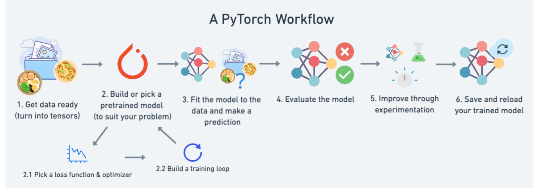
我们现在已经对 01. PyTorch Workflow Fundamentals,我们已经准备好数据,我们已经构建并选择了一个预训练模型,我们已经使用我们的各种辅助函数来训练和评估模型 在这个笔记本中,我们通过运行和跟踪一系列实验改进了我们的 FoodVision Mini 模型。
你应该为自己感到骄傲,这是不小的壮举!
您应该从这个里程碑项目 1 中获得的主要想法是:
• 机器学习从业者的座右铭:实验、实验、实验!
• 在开始时,请保持小规模的实验,以便您可以快速工作。你做的实验越多,你就能越快找出不起作用的东西。
• 当你找到有用的东西时扩大规模。例如我们发现了性能很好的模型,也许您现在想看看当您将其扩展到整个 Food101 数据集(来自
torchvision.datasets
)时会发生什么。• 跟踪您的实验需要进行一些设置,但从长远来看这是值得的,这样您就可以弄清楚哪些有效,哪些无效。
