
前言
数据库将SQL解析成一棵语法树后,就需要将语法树转换成查询树,然而查询树的每一个节点或者节点之间的连接都会有一种或者多种实现算法,而需要从中挑选出最优的节点组合。
路径表示单个表的访问方式(顺序访问、索引访问、点查)、两个表的连接方式(嵌套连接、归并连接、hash连接)以及多个表的连接顺序。 那么优化器需要枚举出所有的路径,从中挑选代价最低的路径来执行。
查询树上有的节点是可以直接进行优化的,如过滤、投影等,在查询树底部先将不需要的数据过滤掉,以减少数据量往查询树上层的传递以及操作的成本,这种优化是显而易见的,是基于经验的,我们称为启发式规则优化。 然而,有的优化是无法直接进行的,例如,A JOIN B
,JOIN顺序A JOIN B
或者 B JOIN A
都会输出正确的查询树结果,哪种顺序成本最低呢,这就需要基于统计数据来进行估算,找出代价最小的顺序,这种优化我们称之为基于成本的优化。
路径选择理论
因为不同的关系访问方式,ORDER、JOIN方式组合和排列非常多,而JOIN的优化是最为复杂的,所以我们就只讨论数据库是如何挑选出最优的JOIN路径的。
JOIN顺序的枚举
对于OUTER JOIN来说,JOIN顺序是固定的,所以路径数量相对较少(只需要考虑不同JOIN算法组成的路径);然而对于INNER JOIN来说,表之间的JOIN顺序是可以不同的,这样就可以由不同的JOIN组合、不同的JOIN顺序组成非常多的不同路径。 如A JOIN B JOIN C
,路径有:
(A⋈B)⋈C :就有两种排列顺序
(A JOIN B) JOIN C
和C JOIN (A JOIN B)(A JOIN C) JOIN BA JOIN (C JOIN B)等等
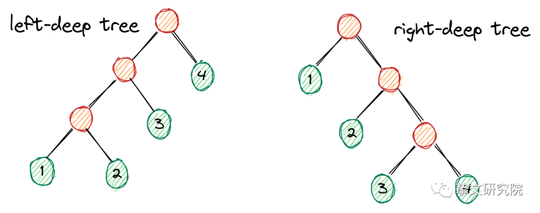
我们将所有join顺序组成的树的形态分为
左深树left-deep tree:((1⋈2)⋈3)⋈4
右深树right-deep tree:1⋈(2⋈(3⋈4))
紧密树bushy tree: (1⋈2)⋈(3⋈4), ((1⋈2)⋈3)⋈(4⋈5)
 JOIN连接的形状 就是一棵full binary tree 的形状,树形态的数量 是一个卡塔兰数(catalan number), 所以就有 $$ C_{n} = \frac{(2(n-1))!}{n!(n-1)!} $$ 种形态的树。
而每种形态的树,都会有n!
种排列, 所以n种关系(表,子查询等)就会有 (2(n − 1))!∕(n − 1)!
种不同的JOIN路径。
例如4个表JOIN,组成的树的形态就有5种,而每种形态 4! 种排列,所以就有5 * 4!=120 种不同的JOIN路径。
如果是7个表连接,就有665280种JOIN路径!那么要将全部的JOIN路径枚举出来,是非常耗时的。
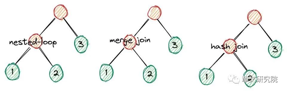
JOIN方式的枚举
JOIN一般有几种实现方式:嵌套连接、归并连接、hash连接等,所以不同的JOIN顺序还有这几种JOIN方式。
如:A⋈B就有两种排列顺序A JOIN B
和 B JOIN A
而根据不同的JOIN方式有:
A nested-loop join BA merge join BA hash join B
实现方式
通常数据库使用以下几种方法来从JOIN路径中找出成本最优的路径
动态规划:考虑全部子集,从中找出最优子集
贪心算法:考虑部分子集
随机算法:考虑部分子集,常见的有模拟退火算法,随机爬山算法,遗传算法等等
动态规划
遍历出所有的路径,记忆路径子集,避免重复计算,通过最优子问题构建出整个问题最优解。这种方法能够计算出最优路径,但是如果表的个数变多,则“基于代价的动态规划算法”暴露出连接膨胀的问题。依据前面的计算,7个表就有665280种连接顺序,就算有大量子问题能避免重复计算,但整个计算成本还是相当巨大的。
如果表太多,我们就要取舍,追求次最优或者局部最优解(尽量扩大局部性),如贪心算法、随机算法
贪心算法
贪心算法求解局部最优解,在局部最优解的基础上再去扩大局部最优解,然而这种方法是具有后效性的,得出的结果不一定是最优的。
随机算法
使用贪心算法,前面子问题的解确定下来后,如果子问题的解导致全局的解不是最优,那么就没有修正的余地了。 而随机算法一般是在局部最优解确定下来后,仍然可以以一定概率进行"变化",以谋求存在一定概率下能打破子问题后效性。
如:遗传算法中,优胜劣汰的规则,会求出局部最优解,但仍然存在一定概率进行"变异",这样可以存在多个局部解,最优解的被选择概率更高,就确保了在子问题最优而全局不是最优的情况下,仍然有一定概率选择其他子问题解,以谋求得到相对更优的全局解。
不同的数据库选用的算法不一样,有的选用贪心,或者动态规划,或者随机退火等等,而postgreSQL的实现较为灵活,当表较少时,选择动态规划,否则选择遗传算法,还可以允许用户自己定义路径算法。
postgreSQL实现
postgreSQL的路径生成算法有三种:
动态规划
遗传算法
用户自定义
路径生成由make_one_rel
函数完成,首先为每个基本关系生成不同的访问路径, 再将这些关系作为叶子节点生成JOIN路径。
RelOptInfo *make_one_rel(PlannerInfo *root, List *joinlist){......// 为每个关系生成不同的访问路径set_base_rel_pathlists(root);// 生成JOIN路径rel = make_rel_from_joinlist(root, joinlist);return rel;}
生成不同访问路径
遍历所有的关系,为关系生成不同访问路径
static void set_base_rel_pathlists(PlannerInfo *root){for (rti = 1; rti < root->simple_rel_array_size; rti++){......set_rel_pathlist(root, rel, rti, root->simple_rte_array[rti]);}}static void set_rel_pathlist(PlannerInfo *root, RelOptInfo *rel, Index rti, RangeTblEntry *rte){......switch (rel->rtekind){// 关系case RTE_RELATION:......else // 普通关系{set_plain_rel_pathlist(root, rel, rte);}......}......set_cheapest(rel);}
再看看普通关系如何生成路径的
static void set_plain_rel_pathlist(PlannerInfo *root, RelOptInfo *rel, RangeTblEntry *rte){......// 顺序扫描路径add_path(rel, create_seqscan_path(root, rel, required_outer, 0));// 是否支持索引扫描,支持则添加到路径中create_index_paths(root, rel);// 表达式是否可以转成TID扫描,create_tidscan_paths(root, rel);}
生成基本访问路径后,就开始进行JOIN路径计算了。
static RelOptInfo *make_rel_from_joinlist(PlannerInfo *root, List *joinlist){......if (levels_needed == 1){ // 只有一个join关系,则直接返回return (RelOptInfo *) linitial(initial_rels);}else{......// 如果有自定义join生成算法则使用if (join_search_hook)return (*join_search_hook) (root, levels_needed, initial_rels);// 如果开启了遗传算法且join关系大于阈值(默认12)则使用遗传算法else if (enable_geqo && levels_needed >= geqo_threshold)return geqo(root, levels_needed, initial_rels);else // 否则,使用动态规划算法return standard_join_search(root, levels_needed, initial_rels);}}
遗传算法
算法
遗传算法:
对问题进行编码,确定搜索空间的大小
随机初始化群体(主要是给染色体赋初始值,计算每个染色体的适应度的值,并对各个染色体的适应度排序),以及计算好进化次数
循环:进行N次进化
“随机”选出两个染色体,分别是momma和daddy
对于momma和daddy使用“杂交”方式,求出其孩子
求杂交得到的kid的适应度的值
把kid插入群体中(如果kid的适应度比群体中最差的适应度还差,则不插入,否则,替换掉最差的那个且排好序)
生成了最优路径
根据最优的连接路径生成查询执行计划和花费估算
实现
种群Pool
用来存储染色体,所有染色体在种群中进化出最终的较优染色体。
typedef struct Pool{Chromosome *data; // 染色体数据int size; // 染色体数量int string_length; // 染色体大小,用以连接的表的数目} Pool;
基因Gene
最小进化单位,在这里定义成基本关系,Relid
typedef int Gene;
染色体Chromosome
由基因组成,且由worth
来表示此染色体的适应度,适应度差的更高的概率会被淘汰掉。
typedef struct Chromosome{Gene *string; // 基因,是连接表构成的序列即一连串不重复的整数形式的字符串Cost worth; // 适应度,也就是路径代价} Chromosome;
postgreSQL实现了几种杂交算法
基于边重组杂交 (edge recombination crossover)
部分匹配杂交 (partially matched crossover)
循环杂交 (cycle crossover)
位置杂交 (position crossover)
顺序杂交 (order crossover)
由于基于边重组杂交是默认的算法,所以我们这里只讨论此算法。
主流程
代码中只保留了基于边重组的杂交算法
RelOptInfo *geqo(PlannerInfo *root, int number_of_rels, List *initial_rels){int generation;Chromosome *momma;Chromosome *daddy;Chromosome *kid;Pool *pool;int pool_size,number_generations;Gene *best_tour;Edge *edge_table; /* list of edges */......// 计算种群大小pool_size = gimme_pool_size(number_of_rels);// 计算杂交次数(进化次数)number_generations = gimme_number_generations(pool_size);// 分配种群pool = alloc_pool(root, pool_size, number_of_rels);// 随机初始化群体(主要是给染色体赋初始值,并调用geqo_eval函数为每个染色体求适应度的值,// 调用sort_pool函数对各个染色体的适应度排序)。random_init_pool(root, pool);// 按照适应度值(cheapestpath)排序群体中的染色体,// 适应度值小表示此路径花费小,应该优先选择sort_pool(root, pool);// 分配父母染色体momma = alloc_chromo(root, pool->string_length);daddy = alloc_chromo(root, pool->string_length);// 创建边表(边重组)edge_table = alloc_edge_table(root, pool->string_length);// 开始进化for (generation = 0; generation < number_generations; generation++){// 选择:利用线性偏差函数,从中选出父母geqo_selection(root, momma, daddy, pool, Geqo_selection_bias);// **基于边重组杂交**// 通过父母染色体来初始化边表gimme_edge_table(root, momma->string, daddy->string, pool->string_length, edge_table);// 分配kid染色体kid = momma;// 杂交 :从边表中选择合适的基因组成新的染色体edge_failures += gimme_tour(root, edge_table, kid->string, pool->string_length);// 计算kid的适应度,通过gimme_tree构造最优路径kid->worth = geqo_eval(root, kid->string, pool->string_length);// 进化:// 将kid插入种群中,如果kid比种群中最差的个体适应度差,则不插入// 否则使用二分查找到合适位置替换掉适应度比kid差的个体spread_chromo(root, kid, pool);}// 把最优路径传递给gimme_treebest_tour = (Gene *) pool->data[0].string;best_rel = gimme_tree(root, best_tour, pool->string_length);......return best_rel;}
确定种群大小
种群越大,理论上就越能找出最优解,但就会导致计算成本的增加,所以要对种群大小进行取舍。
static int gimme_pool_size(int nr_rel){......// 如果指定了群体的大小,指定值大于等于2,则采用指定值为群体大小if (Geqo_pool_size >= 2)return Geqo_pool_size;// size = 2^(nr_rel + 1)size = pow(2.0, nr_rel + 1.0);// 约束maxsize = 50 * Geqo_effort; /* 50 to 500 individuals */if (size > maxsize)return maxsize;minsize = 10 * Geqo_effort; /* 10 to 100 individuals */if (size < minsize)return minsize;return (int) ceil(size);}
初始化种群
随机初始化种群
void random_init_pool(PlannerInfo *root, Pool *pool){......while (i < pool->size){init_tour(root, chromo[i].string, pool->string_length);pool->data[i].worth = geqo_eval(root, chromo[i].string, pool->string_length);if (pool->data[i].worth < DBL_MAX)i++;else{bad++;if (i == 0 && bad >= 10000)elog(ERROR, "geqo failed to make a valid plan");}}}
生成染色体
改进的Fisher-Yates洗牌算法, 利用了编码有序的特点,将初始化染色体和随机交换结合起来一起进行
// 随机生成连接顺序void init_tour(PlannerInfo *root, Gene *tour, int num_gene){......if (num_gene > 0)tour[0] = (Gene) 1;for (i = 1; i < num_gene; i++){j = geqo_randint(root, i, 0);// 交换i和j的值(i并没有初始化)/* i != j check avoids fetching uninitialized array element */if (i != j)tour[i] = tour[j]; //将tour[j]的值赋值给tour[i]tour[j] = (Gene) (i + 1); // tour[i]之前的值(初始化)赋值给tour[j]}}
适应度
geqo_eval
函数的主要只有两步
通过
gimme_tree
函数进行多表连接计算连接结果的适应度值
Cost geqo_eval(PlannerInfo *root, Gene *tour, int num_gene){......// 进行多表连接joinrel = gimme_tree(root, tour, num_gene);if (joinrel){ // 计算连接结果的适应度Path *best_path = joinrel->cheapest_total_path;fitness = best_path->total_cost;}elsefitness = DBL_MAX;......return fitness;}
选择染色体
由于种群中的染色体已经按照适应度排好序了,对我们来说适应度越低(代价越低)的染色体越好,因此选择操作基于概率分布的随机。 这样在选择父亲染色体和母亲染色体的时候更倾向于选择适应度低的染色体,同时也有机会选择非局部最优染色体,以达到能够一定随机性。
void geqo_selection(PlannerInfo *root, Chromosome *momma, Chromosome *daddy, Pool *pool, double bias){int first,second;// 选择两个随机数(基于概率分布的)first = linear_rand(root, pool->size, bias);second = linear_rand(root, pool->size, bias);......// 在种群中基于随机数选择父母染色体geqo_copy(root, momma, &pool->data[first], pool->string_length);geqo_copy(root, daddy, &pool->data[second], pool->string_length);}
线性随机
static int linear_rand(PlannerInfo *root, int pool_size, double bias){double index; /* index between 0 and pool_size */double max = (double) pool_size;do{double sqrtval;sqrtval = (bias * bias) - 4.0 * (bias - 1.0) * geqo_rand(root);if (sqrtval > 0.0)sqrtval = sqrt(sqrtval);index = max * (bias - sqrtval) 2.0 (bias - 1.0);} while (index < 0.0 || index >= max);return (int) index;}
先生成一个基于[0, 1]之间的随机值,然后根据概率分布函数求出符合概率密度的随机值。
生成基于某种概率分布的随机数,要先计算其概率密度函数,postgreSQL的概率密度函数为
$$ f(x) = bias - 2(bias -1)x, (0<x<1) $$
bias默认是2,所以 概率密度函数 f(x) = 2-2x
,代表概率的变化率。
通过概率密度函数获得概率分布函数
$$ F(x) = \int f(x)dx = bias \times x - (bias - 1) \times x^2, (0<x<1) $$
通过概率分布函数的逆函数法可以获得符合概率分布的随机数
$$ F^{-1}(x) = \frac{bias - \sqrt{bias^2 - 4(bias - 1)y}}{2(bias - 1)} $$
求得概率分布函数如图中红色曲线, 概率分布函数逆函数如图中蓝线,
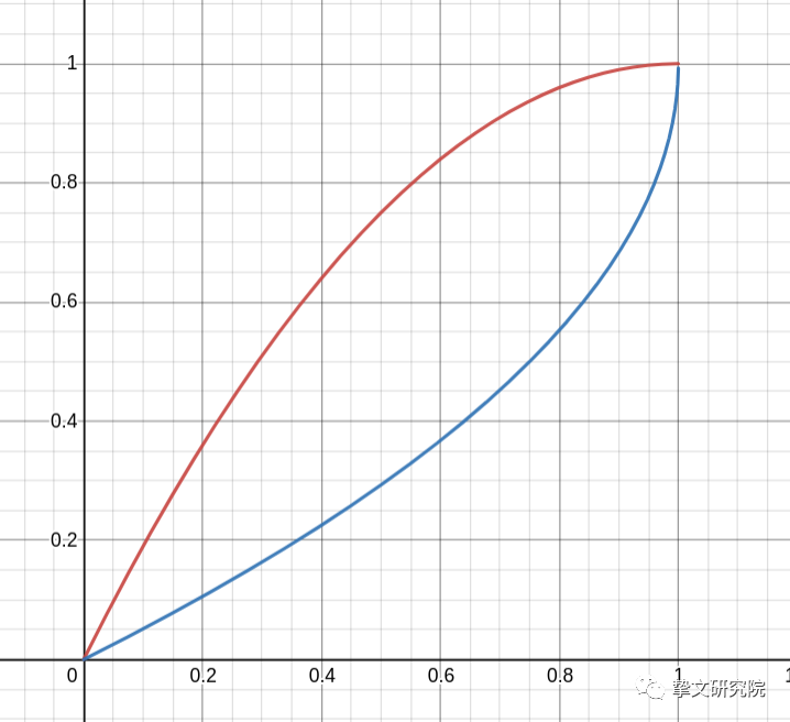
从图中红色曲线可以看出,在X轴上递增,则概率越低(连续型随机变量)。如:F(x)d(0 ~ 0.2)的概率就比F(x)d(0.4 ~ 0.6)高。
而蓝色曲线是概率分布函数的逆函数,值域(Y轴)为随机变量,在X轴上选定任意的p(0<=p<=1)时,通过逆函数得到的是随机变量的值,也就是获得概率和为p的随机变量的上限。所以通过逆函数,可以将rand(0, 1)
“转换成” 符合概率密度分布的随机值。
测试:将linear_rand代码提取出来,进化10000次,种群选择10,那么10条染色体被选中的概率分别为18.8%,16.9%,15.5%,12.9%,11.3%,9.3%,6.3%,5.1%,2.8%,1.1%,可以看出概率变化是符合概率密度函数 f(x) = 2-2x
的。
bias的选择
密度函数中bias越大,则适应度低的染色体被选择概率更高,随着进化次数越多,产生"近亲繁殖"的概率就越高,也就越容易造成贪心算法类似的问题;bias越小,则"优胜劣汰"的速度越慢,需要的进化次数越多,但是,最终找出最优解的可能性也越高。
杂交算法
默认的杂交算法是:基于边重组的杂交。
算法
如2条染色体
染色体1:(A, D, C, B)
染色体2:(C, B, D, A)
边关系
视染色体为循环队列:染色体1中A与B是有边关系的
边关系是双向的:如染色体1中,基因A和D的边关系为(A, D)和(D, A)
我们使用一个边表来存储染色体的基因之间的边关系
A -> (-D, B, C) : 表示基因A和(D, B, C)有边关系,而(-D)表示有2条这样的边关系,称为共享边
B -> (A, -C, D)
C -> (D, -B, A)
D -> (-A, C, B)
在交叉过程中,会尽量选择共享边,这样可以达到选择较优基因的目的。
边表
边表用来存储染色体中基因的边关系。
typedef struct Edge{Gene edge_list[4]; // 每个基因有4条边(2条染色体,前后左右各2条)int total_edges; // 总的数量int unused_edges; // 没有选择的边数量} Edge;
alloc_edge_table
分配表边,为总数=基因+1
的边。
根据染色体来填充边表
// tour1和tour2为2条染色体float gimme_edge_table(PlannerInfo *root, Gene *tour1, Gene *tour2, int num_gene, Edge *edge_table){......// index1和index2为2个基因的索引for (index1 = 0; index1 < num_gene; index1++){//index2 = (index1 + 1) % num_gene;// 边是双向的,填充1->2,也填充2->1// 填充tour1染色体的边关系edge_total += gimme_edge(root, tour1[index1], tour1[index2], edge_table);gimme_edge(root, tour1[index2], tour1[index1], edge_table);// 填充tour2染色体的边关系edge_total += gimme_edge(root, tour2[index1], tour2[index2], edge_table);gimme_edge(root, tour2[index2], tour2[index1], edge_table);}return ((float) (edge_total * 2) (float) num_gene);}static int gimme_edge(PlannerInfo *root, Gene gene1, Gene gene2, Edge *edge_table){int i;int edges;int city1 = (int) gene1;int city2 = (int) gene2;// edge_list: city1指向的基因的边,如基因A->B,A->C, A->M,edges存储[B,C,M]// 边数量edges = edge_table[city1].total_edges;// 如果基因city1->city2已经存在,说明其他染色体也有此边关系// 则在city1的edge_list中city2改写成 -city2,// 即[-B, C, M],表示这是共享边for (i = 0; i < edges; i++){if ((Gene) Abs(edge_table[city1].edge_list[i]) == city2){edge_table[city1].edge_list[i] = 0 - city2;return 0;}}// 添加city1->city2边关系edge_table[city1].edge_list[edges] = city2;edge_table[city1].total_edges++;edge_table[city1].unused_edges++;return 1;}
通过边表,生成新的染色体
int gimme_tour(PlannerInfo *root, Edge *edge_table, Gene *new_gene, int num_gene){int i;int edge_failures = 0;// 随机选择一个基因new_gene[0] = (Gene) geqo_randint(root, num_gene, 1);for (i = 1; i < num_gene; i++){// 将边表中,指向new_gene[i-1]的边删除掉remove_gene(root, new_gene[i - 1], edge_table[(int) new_gene[i - 1]], edge_table);// 如果new_gene[i-1]的edge_list中还有边关系,则从中找一个比较"合适"的边关系if (edge_table[new_gene[i - 1]].unused_edges > 0)new_gene[i] = gimme_gene(root, edge_table[(int) new_gene[i - 1]], edge_table);else{ // 如果new_gene[i-1]的edge_list中国没有边关系,则随机找一个new_gene中没有的基因edge_failures++;new_gene[i] = edge_failure(root, new_gene, i - 1, edge_table, num_gene);}edge_table[(int) new_gene[i - 1]].unused_edges = -1;} /* for (i=1; i<num_gene; i++) */return edge_failures;}
从基因的边关系中找出一条“合适的”边关系
优先选择共享边关系:共享边是指某条边在父母中都存在,也说明2个基因组成的这条边是较优的,所以要尽量继承下去。
从邻居基因的边关系中,找出其边关系最少的邻居
static Gene gimme_gene(PlannerInfo *root, Edge edge, Edge *edge_table){......minimum_edges = 5;// 遍历边关系for (i = 0; i < edge.unused_edges; i++){friend = (Gene) edge.edge_list[i];// 优先选择共享边if (friend < 0)return (Gene) Abs(friend);// 在所有邻居基因中,找出边关系最少的if (edge_table[(int) friend].unused_edges < minimum_edges){minimum_edges = edge_table[(int) friend].unused_edges;minimum_count = 1;}else if (minimum_count == -1)elog(ERROR, "minimum_count not set");else if (edge_table[(int) friend].unused_edges == minimum_edges)minimum_count++;}rand_decision = geqo_randint(root, minimum_count - 1, 0);// 在"边关系最少的"邻居基因中随机选择一个for (i = 0; i < edge.unused_edges; i++){friend = (Gene) edge.edge_list[i];/* return the chosen candidate point */if (edge_table[(int) friend].unused_edges == minimum_edges){minimum_count--;if (minimum_count == rand_decision)return friend;}}elog(ERROR, "neither shared nor minimum number nor random edge found");return 0; /* to keep the compiler quiet */}
这样,我们就通过边重组的方式,产生出较优的染色体。
生成连接路径
根据指定的染色体,生成最佳路径。
RelOptInfo *gimme_tree(PlannerInfo *root, Gene *tour, int num_gene){......clumps = NIL;// 遍历所有基因for (rel_count = 0; rel_count < num_gene; rel_count++){......// 提取关系, Get the next input relationcur_rel_index = (int) tour[rel_count];cur_rel = (RelOptInfo *) list_nth(private->initial_rels, cur_rel_index - 1);/* Make it into a single-rel clump */cur_clump = (Clump *) palloc(sizeof(Clump));cur_clump->joinrel = cur_rel;cur_clump->size = 1;// clumps初始是NIL,不断增加可做连接的连接后的关系。// merge_clump函数的作用就是把cur_clump和clumps中的每个可连接的关系进行连接,// 连接的结果放于clumps中/* Merge it into the clumps list, using only desirable joins */clumps = merge_clump(root, clumps, cur_clump, num_gene, false);}if (list_length(clumps) > 1){/* Force-join the remaining clumps in some legal order */List *fclumps;ListCell *lc;fclumps = NIL;foreach(lc, clumps){Clump *clump = (Clump *) lfirst(lc);fclumps = merge_clump(root, fclumps, clump, num_gene, true);}clumps = fclumps;}/* Did we succeed in forming a single join relation? */if (list_length(clumps) != 1)return NULL;return ((Clump *) linitial(clumps))->joinrel;}
new_clump与clumps中每项进行连接,如果可以连接(且连接顺序符合染色体), 则连接并加入到clumps中,如果不可以,则将new_clump加入到clumps中。
static List *merge_clump(PlannerInfo *root, List *clumps, Clump *new_clump, int num_gene, bool force){ListCell *lc;int pos;foreach(lc, clumps){Clump *old_clump = (Clump *) lfirst(lc);if (force || desirable_join(root, old_clump->joinrel, new_clump->joinrel)){RelOptInfo *joinrel;// 完成关系连接处理joinrel = make_join_rel(root, old_clump->joinrel, new_clump->joinrel);if (joinrel){generate_partitionwise_join_paths(root, joinrel);if (old_clump->size + new_clump->size < num_gene)generate_useful_gather_paths(root, joinrel, false);// 找关系上的最优路径/* Find and save the cheapest paths for this joinrel */set_cheapest(joinrel);old_clump->joinrel = joinrel;old_clump->size += new_clump->size;pfree(new_clump);/* Remove old_clump from list */// 去掉old_clump,保证下步递归调用merge_clump函数时不和自身连接clumps = foreach_delete_current(clumps, lc);return merge_clump(root, clumps, old_clump, num_gene, force);}}}if (clumps == NIL || new_clump->size == 1)return lappend(clumps, new_clump);for (pos = 0; pos < list_length(clumps); pos++){Clump *old_clump = (Clump *) list_nth(clumps, pos);if (new_clump->size > old_clump->size)break;}clumps = list_insert_nth(clumps, pos, new_clump);return clumps;}
动态规划
算法
过程
第一步 : 初始化第1层关系,为基本关系节点,包含基本关系的数据访问路径
第二步 :生成第2层到第n层关系:
左右深树连接方式:将第2层到第n-1层的每个关系,与第1层中的每个关系连接,生成新的关系,每一个新关系,均求出最优路径
紧密树连接方式:将第k层(2<=k<=n-k)的每个关系,与第other_level层(n-k)中的每个关系连接,生成新的关系放于第n层,且每一个新关系,均求解其最优路径
实现
主流程
RelOptInfo *standard_join_search(PlannerInfo *root, int levels_needed, List *initial_rels){......// 第1层// 每个节点是一个基本关系(包含每个关系的所有访问方式)root->join_rel_level[1] = initial_rels;// 从第2层开始,求出每层的连接关系for (lev = 2; lev <= levels_needed; lev++){// 计算出第k层所有的中间关系join_search_one_level(root, lev);// 遍历lev上每个中间关系,找出最优的foreach(lc, root->join_rel_level[lev]){rel = (RelOptInfo *) lfirst(lc);......// 查找本节点最优路径set_cheapest(rel);}}// 返回最终路径rel = (RelOptInfo *) linitial(root->join_rel_level[levels_needed]);root->join_rel_level = NULL;return rel;}
计算某层的中间关系
左右深树
PlannerInfo
结构上的join_rel_level
的用来存储关系,第1层是基本表关系,第2层到第N层是连接关系。
假设A JOIN B JOIN C JOIN D
,join_rel_level
如下:
join_rel_level[1]:(A),(B),(C),(D)
join_rel_level[2]:连接第1层的表(满足JOIN约束),得到(A⋈B),(A⋈C),(A⋈D),(B⋈C),(B⋈D),(C⋈D)
(A⋈B) :路径有(A JOIN B), (B JOIN A) 两种join顺序,
A merge-join B
,A hash-join B
等不同的join方式。join_rel_level[3]:用第1层和第2层的关系连接得到
左深树: ((A⋈B)⋈C),((A⋈B)⋈D),((A⋈C)⋈D),((B⋈C)⋈D) ,等等
右深树:(A⋈(B⋈C)), (A⋈(B⋈D))等等
join_rel_level[4]:用第3层和第1层的关系进行连接
(((A⋈B)⋈C)⋈D), (A⋈(B⋈(C⋈D))) 等等
最终生成整个问题的最优路径。
紧密树
紧密树是由两个或多个连接关系之间再进行连接产生的关系。
所以,只有大于3层的关系才能产生紧密树,假如A JOIN B JOIN C JOIN D JOIN E
将第2层之间进行连接:((A⋈B)⋈(C⋈D)), ((A⋈D)⋈(B⋈C)), ((D⋈E)⋈(B⋈C)) 等
将第2层与第3层进行连接:((A⋈B)⋈(C⋈(D⋈E))),
// 计算出level的节点void join_search_one_level(PlannerInfo *root, int level){......// 左深树和右深树// 遍历下一层的所有节点,将其与第1层节点进行JOINforeach(r, joinrels[level - 1]){RelOptInfo *old_rel = (RelOptInfo *) lfirst(r);// 符合连接约束if (old_rel->joininfo != NIL || old_rel->has_eclass_joins ||has_join_restriction(root, old_rel)){......other_rels_list = joinrels[1]; // 第1层relsother_rels = list_head(other_rels_list); // 第1层的第一个rel或者当level=2时,第1层中r后面的rels,避免重复计算// 找出所有old_rel 和 other_rels_list的other_rels节点以后所有节点的 的连接make_rels_by_clause_joins(root, old_rel, other_rels_list, other_rels);}else // 没有join关系,做笛卡尔积{make_rels_by_clauseless_joins(root, old_rel, joinrels[1]);}}// bushy join,用第k层和level-k层连接,构成第level层关系; 而level在本函数的上层函数,// 是从2到N从小到大动态变化的,这样,逐步对每层能够利用bushy连接方式构造连接树for (k = 2;; k++){int other_level = level - k;if (k > other_level)break;// 遍历第k层节点foreach(r, joinrels[k]){......// 遍历level-k层节点for_each_cell(r2, other_rels_list, other_rels){RelOptInfo *new_rel = (RelOptInfo *) lfirst(r2);if (!bms_overlap(old_rel->relids, new_rel->relids)){if (have_relevant_joinclause(root, old_rel, new_rel) ||have_join_order_restriction(root, old_rel, new_rel)){(void) make_join_rel(root, old_rel, new_rel);}}}}}// 如果没有连接则做cartesian-product,if (joinrels[level] == NIL){......}}// old_rel与 other_rels 之间生成连接关系static void make_rels_by_clause_joins(PlannerInfo *root, RelOptInfo *old_rel, List *other_rels_list, ListCell *other_rels){ListCell *l;for_each_cell(l, other_rels_list, other_rels){RelOptInfo *other_rel = (RelOptInfo *) lfirst(l);// 两个relis没有相同的relation,且有join关联性,且符合join顺序要求if (!bms_overlap(old_rel->relids, other_rel->relids) &&(have_relevant_joinclause(root, old_rel, other_rel) ||have_join_order_restriction(root, old_rel, other_rel))){(void) make_join_rel(root, old_rel, other_rel);}}}
创建关系
make_join_rel
用于创建一个新的连接关系并生成此连接关系的路径。
这个新关系的构成的每种方式就是一个路径,并保存于RelOptInfo
的pathlist
。
RelOptInfo *make_join_rel(PlannerInfo *root, RelOptInfo *rel1, RelOptInfo *rel2){......// 查找joinrel,如果没有则创建一个joinrel = build_join_rel(root, joinrelids, rel1, rel2, sjinfo, &restrictlist);......// 生成路径populate_joinrel_with_paths(root, rel1, rel2, joinrel, sjinfo, restrictlist);bms_free(joinrelids);return joinrel;}RelOptInfo *build_join_rel(PlannerInfo *root, Relids joinrelids, RelOptInfo *outer_rel, RelOptInfo *inner_rel, SpecialJoinInfo *sjinfo, List **restrictlist_ptr){......// 先查找此连接关系是否已经存在,joinrel = find_join_rel(root, joinrelids);if (joinrel){if (restrictlist_ptr)*restrictlist_ptr = build_joinrel_restrictlist(root, joinrel, outer_rel, inner_rel);return joinrel;}// 不存在,则初始化一个joinrel = makeNode(RelOptInfo);joinrel->reloptkind = RELOPT_JOINREL;......return joinrel;}
生成路径
static void populate_joinrel_with_paths(PlannerInfo *root, RelOptInfo *rel1,RelOptInfo *rel2, RelOptInfo *joinrel, SpecialJoinInfo *sjinfo, List *restrictlist){switch (sjinfo->jointype){case JOIN_INNER:......// 生成 (rel1 JOIN rel2) and (rel2 JOIN rel1)两种路径add_paths_to_joinrel(root, joinrel, rel1, rel2, JOIN_INNER, sjinfo, restrictlist);add_paths_to_joinrel(root, joinrel, rel2, rel1, JOIN_INNER, sjinfo, restrictlist);break;case JOIN_LEFT:......// 对于left join:生成(rel1 left join rel2) and (rel2 right join rel1)两种路径add_paths_to_joinrel(root, joinrel, rel1, rel2, JOIN_LEFT, sjinfo, restrictlist);add_paths_to_joinrel(root, joinrel, rel2, rel1, JOIN_RIGHT, sjinfo, restrictlist);break;......}......}
总结
要枚举出查询树上所有路径,从中找出一个代价最小的路径,是个NP问题,计算成本是非常高昂的。而当查询树的关系(表、子查询等)较少时,可以使用动态规划算法枚举出所有的路径找出最优解,但是当关系较多时,枚举的计算成本是我们无法接受的,这时就需要使用一些折中方案,如贪心算法、遗传算法。遗传算法借鉴自然界“优胜劣汰”的法则对路径进化,从而能找出相对较优的查询路径。

PCP 认 证 专 家 报 名