失衡数据采样方法

细说数据 2021-06-28

3208

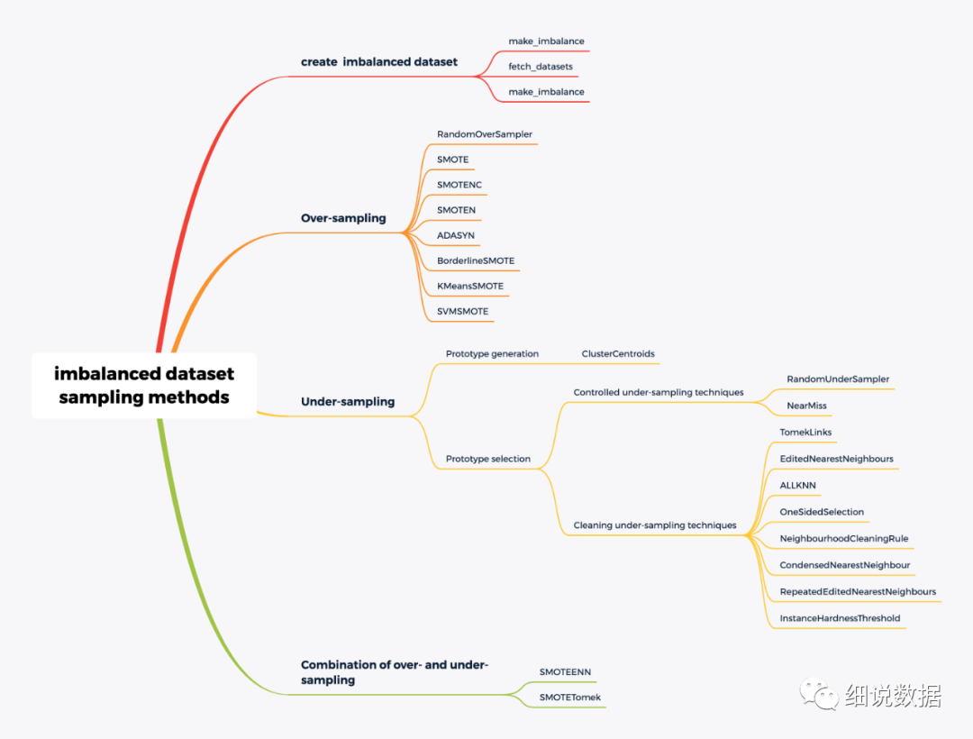
j所谓的不平衡指的是不同类别的样本量异非常大。针对不平衡数据, 最简单的一种方法就是欠采样和过采样。

1、生成不平衡数据集

生成不平衡数据集的方法有三种make_imbalance、fetch_datasets、make_classification

make_imbalance

将数据集转换为具有特定采样策略的不平衡数据集

imblearn.datasets.make_imbalance(X, y, *, sampling_strategy=None, 
random_state=None, verbose=False, **kwargs)

X：包含不平衡数据的矩阵。

y：X 中每个样本的对应标签。

sampling_strategy：用于重新采样数据集的比率，可以写成一个字典

random_state：随机数生成器使用的种子

from collections import Counter
from sklearn.datasets import load_iris
from imblearn.datasets import make_imbalance
data = load_iris()
X, y = data.data, data.target
print(f'Distribution before imbalancing: {Counter(y)}')
X_res, y_res = make_imbalance(X, y,
                              sampling_strategy={0: 10, 1: 20, 2: 30},
                              random_state=42)
print(f'Distribution after imbalancing: {Counter(y_res)}')

结果：

Distribution before imbalancing: Counter({0: 50, 1: 50, 2: 50})
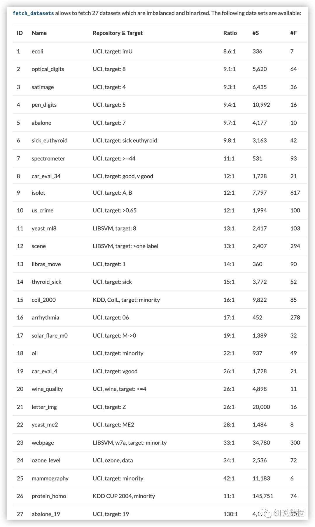
Distribution after imbalancing: Counter({2: 30, 1: 20, 0: 10})

fetch_datasets

scikit-learn 的 datasets 模块大规模数据集

imblearn.datasets.fetch_datasets( * , data_home = None , 
filter_data = None , download_if_missing = True , 
random_state = None , shuffle = False , verbose = False )

data_home：为数据集指定另一个下载和缓存文件夹。默认情况下，所有 scikit-learn 数据都存储在“/scikit_learn_data”子文件夹中

filter_data：含要返回的数据集的 ID 或名称的元组。参考下表获取数据集的ID和名称。

download_if_missing：如果为 False，如果数据在本地不可用，而不是尝试从源站点下载数据，则引发 IOError

random_state：用于混洗数据集的随机状态

shuffle：是否打乱数据集

verbose：显示有关提取的信息

from collections import Counter
from imblearn.datasets import fetch_datasets
ecoli = fetch_datasets()['ecoli']
ecoli.data.shape
print (sorted(Counter(ecoli.target).items()))

make_classification

分类数据生成器

sklearn.datasets.make_classification(n_samples=100, n_features=20, 
*, n_informative=2, n_redundant=2, n_repeated=0,n_classes=2,
n_clusters_per_class=2, weights=None, flip_y=0.01,class_sep=1.0,
hypercube=True, shift=0.0, scale=1.0, shuffle=True, random_state=None)

n_samples：样本数量

n_features：特征个数= n_informative + n_redundant + n_repeated

n_informative：信息特征的数量

n_redundant：冗余特征的数量。这些特征是作为信息特征的随机线性组合生成的。

n_repeated：从信息和冗余特征中随机抽取的重复特征的数量。

n_classes：分类的类别

n_clusters_per_clas：每个类的簇数

weights：分配给每个类的样本比例。

flip_y：其类别被随机分配的样本的比例，默认值 = 0.01

class_sep：乘以超立方体大小的因子。较大的值会分散集群/类并使分类任务更容易。默认值 = 1.0

hypercube：超立方体，如果为 True，则将簇放在超立方体的顶点上。如果为 False，则将簇放在随机多面体的顶点上。默认值 = True

shift：按指定值移动要素。

scale：缩放，将要素乘以指定的值。默认值 = 1.0

shuffle：打乱样本和特征。默认值=True

random_state：生成随机数。

from sklearn.datasets import make_classification
from collections import Counter
X, y = make_classification(n_samples=5000, n_features=2, n_informative=2,
n_redundant=0, n_repeated=0, n_classes=3,
n_clusters_per_class=1,
weights=[0.01, 0.05, 0.94],
class_sep=0.8, random_state=0)
Counter(y)

结果：Counter({2: 4674, 1: 262, 0: 64})

二、过采样：

RandomOverSampler
原理：从样本少的类别中随机抽样，再将抽样得来的样本添加到数据集中。
缺点：重复采样容易导致严重的过拟合

from sklearn.datasets import make_classification
X, y = make_classification(n_samples=5000, n_features=2, n_informative=2,
                            n_redundant=0, n_repeated=0, n_classes=3,
                            n_clusters_per_class=1,
                            weights=[0.01, 0.05, 0.94],
                            class_sep=0.8, random_state=0)
from imblearn.over_sampling import RandomOverSampler
ros = RandomOverSampler(random_state=0)
X_resampled, y_resampled = ros.fit_resample(X, y)
from collections import Counter
print(sorted(Counter(y_resampled).items()))

结果：[(0, 4674), (1, 4674), (2, 4674)]

除了带有替换的随机抽样外，还有两种流行的对少数类进行过采样的方法：（i）合成少数过采样技术（SMOTE）和（ii）自适应合成（ADASYN）采样方法

SMOTE

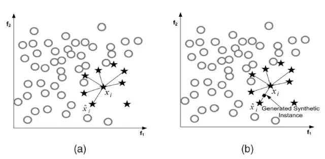
原理：在少数类样本之间进行插值来产生额外的样本。对于少数类样本a, 随机选择一个最近邻的样本b, 从a与b的连线上随机选取一个点c作为新的少数类样本。

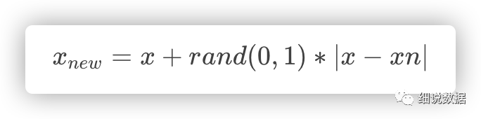
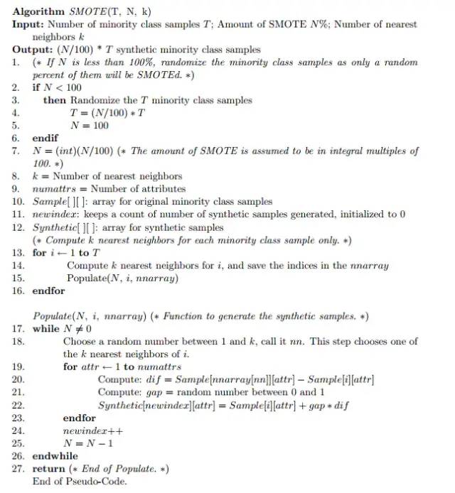
算法流程：1、对于少数类中每一个样本x，以欧氏距离为标准计算它到少数类样本集中所有样本的距离，得到其k近邻。2、根据样本不平衡比例设置一个采样比例以确定采样倍率N，对于每一个少数类样本x，从其k近邻中随机选择若干个样本，假设选择的近邻为xn。3、对于每一个随机选出的近邻xn，分别与原样本按照如下的公式构建新的样本

SMOTE会随机选取少数类样本用以合成新样本，而不考虑周边样本的情况，这样容易带来两个问题：

1）如果选取的少数类样本周围也都是少数类样本，则新合成的样本不会提供太多有用信息。

2）如果选取的少数类样本周围都是多数类样本，这类的样本可能是噪音，则新合成的样本会与周围的多数类样本产生大部分重叠，致使分类困难。

imblearn.over_sampling.SMOTE(*, sampling_strategy='auto', 
random_state=None, k_neighbors=5, n_jobs=None)

sampling_strategy：用于重新采样数据集的比率

random_state：生成随机数

from sklearn.datasets import make_classification
from imblearn.over_sampling import SMOTE 
X, y = make_classification(n_classes=2, class_sep=2,
weights=[0.1, 0.9], n_informative=3, n_redundant=1, flip_y=0,
n_features=20, n_clusters_per_class=1, n_samples=1000, random_state=10)
print('Original dataset shape %s' % Counter(y))
sm = SMOTE(random_state=42)
X_res, y_res = sm.fit_resample(X, y)
print('Resampled dataset shape %s' % Counter(y_res))

结果：Original dataset shape Counter({1: 900, 0: 100})

Resampled dataset shape Counter({0: 900, 1: 900})

SMOTENC

SMOTENC仅当数据混合了数值和分类特征时才有效，如果数据仅由分类数据组成，则可以使用SMOTEN变体。

imblearn.over_sampling.SMOTENC（categorical_features , * , 
sampling_strategy = 'auto' , random_state = None , k_neighbors = 5 , n_jobs = None）

categorical_features：指定哪些特征是分类的

sampling_strategy：少数类中的样本数与多数类中的样本数的期望比率

random_state：随机数发生器

k_neighbors：构建合成样本的最近邻居数

n_jobs：交叉验证循环期间使用的 CPU 内核数

from collections import Counter
from numpy.random import RandomState
from sklearn.datasets import make_classification
from imblearn.over_sampling import SMOTENC
X, y = make_classification(n_classes=2, class_sep=2,
weights=[0.1, 0.9], n_informative=3, n_redundant=1, flip_y=0,
n_features=20, n_clusters_per_class=1, n_samples=1000, random_state=10)
print(f'Original dataset shape {X.shape}')
print(f'Original dataset samples per class {Counter(y)}')
# simulate the 2 last columns to be categorical features
X[:, -2:] = RandomState(10).randint(0, 4, size=(1000, 2))
sm = SMOTENC(random_state=42, categorical_features=[18, 19])
X_res, y_res = sm.fit_resample(X, y)
print(f'Resampled dataset samples per class {Counter(y_res)}')

结果：Original dataset shape (1000, 20)

Original dataset samples per class Counter({1: 900, 0: 100})
Resampled dataset samples per class Counter({0: 900, 1: 900})

SMOTEN

重新采样的数据仅由分类特征组成。

imblearn.over_sampling.SMOTEN（*，sampling_strategy = 'auto'，
random_state = None，k_neighbors = 5，n_jobs = None）

sampling_strategy：少数类中的样本数与多数类中的样本数的期望比率

random_state：随机数发生器

k_neighbors：构建合成样本的最近邻居数

n_jobs：交叉验证循环期间使用的 CPU 内核数

import numpy as np
X = np.array(["A"] * 10 + ["B"] * 20 + ["C"] * 30, dtype=object).reshape(-1, 1)
y = np.array([0] * 20 + [1] * 40, dtype=np.int32)
from collections import Counter
print(f"Original class counts: {Counter(y)}")
from imblearn.over_sampling import SMOTEN
sampler = SMOTEN(random_state=0)
X_res, y_res = sampler.fit_resample(X, y)
print(f"Class counts after resampling {Counter(y_res)}")

结果：Original class counts: Counter({1: 40, 0: 20})

Class counts after resampling Counter({0: 40, 1: 40})

ADASYN

ADASYN名为自适应合成抽样(Adaptive Synthetic Sampling)，其最大的特点是采用某种机制自动决定每个少数类样本需要产生多少合成样本，而不是像SMOTE那样对每个少数类样本合成同数量的样本。ADASYN的缺点是易受离群点的影响，如果一个少数类样本的K近邻都是多数类样本，则其权重会变得相当大，进而会在其周围生成较多的样本。

imblearn.over_sampling.ADASYN（*，sampling_strategy = 'auto'，
random_state = None，n_neighbors = 5，n_jobs = None

sampling_strategy：少数类中的样本数与多数类中的样本数的期望比率

random_state：随机数发生器

n_neighbors 构建合成样本的最近邻居数

n_jobs：交叉验证循环期间使用的 CPU 内核数

from collections import Counter
from sklearn.datasets import make_classification
from imblearn.over_sampling import ADASYN 
X, y = make_classification(n_classes=2, class_sep=2,
weights=[0.1, 0.9], n_informative=3, n_redundant=1, flip_y=0,
n_features=20, n_clusters_per_class=1, n_samples=1000,
random_state=10)
print('Original dataset shape %s' % Counter(y))
ada = ADASYN(random_state=42)
X_res, y_res = ada.fit_resample(X, y)
print('Resampled dataset shape %s' % Counter(y_res))

结果：Original dataset shape Counter({1: 900, 0: 100})

Resampled dataset shape Counter({0: 904, 1: 900})

BorderlineSMOTE

这个算法会先将所有的少数类样本分成三类，如下图所示：
“noise” ：所有的k近邻个样本都属于多数类
“danger” ：超过一半的k近邻样本属于多数类
“safe”：超过一半的k近邻样本属于少数类

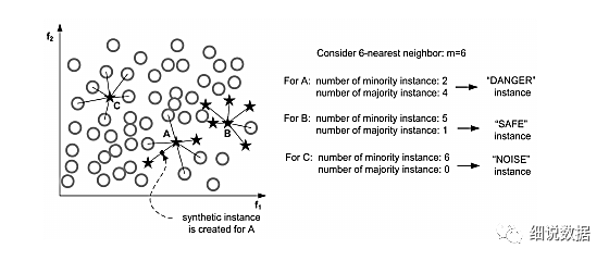
Border-line SMOTE算法只会从处于”danger“状态的样本中随机选择，然后用SMOTE算法产生新的样本。处于”danger“状态的样本代表靠近”边界“附近的少数类样本，而处于边界附近的样本往往更容易被误分类。因而 Border-line SMOTE 只对那些靠近”边界“的少数类样本进行人工合成样本，而 SMOTE 则对所有少数类样本一视同仁。

Border-line SMOTE 分为两种: Borderline-1 SMOTE 和 Borderline-2 SMOTE。Borderline-1 SMOTE 在合成样本时式中的x^是一个少数类样本，而 Borderline-2 SMOTE 中的x^则是k近邻中的任意一个样本。

imblearn.over_sampling.BorderlineSMOTE（*，sampling_strategy = 'auto'，
random_state = None，k_neighbors = 5，n_jobs = None，
m_neighbors = 10，kind = 'borderline-1'）

sampling_strategy：少数类中的样本数与多数类中的样本数的期望比率

random_state：随机数发生器

k_neighbors：构建合成样本的最近邻居数

n_jobs：交叉验证循环期间使用的 CPU 内核数

m_neighbors：则用于确定少数样本是否处于危险中的最近邻居数

kind：使用以下选项之一的 SMOTE 算法类型：'borderline-1', 'borderline-2'

from collections import Counter
from sklearn.datasets import make_classification
from imblearn.over_sampling import BorderlineSMOTE 
X, y = make_classification(n_classes=2, class_sep=2,
weights=[0.1, 0.9], n_informative=3, n_redundant=1, flip_y=0,
n_features=20, n_clusters_per_class=1, n_samples=1000, random_state=10)
print('Original dataset shape %s' % Counter(y))
sm = BorderlineSMOTE(random_state=42)
X_res, y_res = sm.fit_resample(X, y)
print('Resampled dataset shape %s' % Counter(y_res))

结果：Original dataset shape Counter({1: 900, 0: 100})

Resampled dataset shape Counter({0: 900, 1: 900})

KMeansSMOTE

在使用SMOTE进行过采样之前应用KMeans聚类。

KMeansSMOTE包括三个步骤：聚类、过滤和过采样。在聚类步骤中，使用k均值聚类为k个组。过滤选择用于过采样的簇，保留具有高比例的少数类样本的簇。然后，它分配合成样本的数量，将更多样本分配给少数样本稀疏分布的群集。最后，过采样步骤，在每个选定的簇中应用SMOTE以实现少数和多数实例的目标比率。

imblearn.over_sampling.KMeansSMOTE（*，sampling_strategy = 'auto'，
random_state = None，k_neighbors = 2，n_jobs = None，kmeans_estimator = None，
cluster_balance_threshold = 'auto'，density_exponent = 'auto'）

sampling_strategy：少数类中的样本数与多数类中的样本数的期望比率

random_state：随机数发生器

k_neighbors：构建合成样本的最近邻居数

n_jobs：交叉验证循环期间使用的 CPU 内核数

kmeans_estimator：一个 KMeans 实例或要使用的集群数量

cluster_balance_threshold：SMOTE 选择的类的样本将被过采样的阈值

import numpy as np
from imblearn.over_sampling import KMeansSMOTE
from sklearn.datasets import make_blobs
blobs = [100, 800, 100]
X, y  = make_blobs(blobs, centers=[(-10, 0), (0,0), (10, 0)])
# Add a single 0 sample in the middle blob
X = np.concatenate([X, [[0, 0]]])
y = np.append(y, 0)
# Make this a binary classification problem
y = y == 1
sm = KMeansSMOTE(random_state=42)
X_res, y_res = sm.fit_resample(X, y)
# Find the number of new samples in the middle blob
n_res_in_middle = ((X_res[:, 0] > -5) & (X_res[:, 0] < 5)).sum()
print("Samples in the middle blob: %s" % n_res_in_middle)
print("Middle blob unchanged: %s" % (n_res_in_middle == blobs[1] + 1))
print("More 0 samples: %s" % ((y_res == 0).sum() > (y == 0).sum()))

结果：Samples in the middle blob: 801

Middle blob unchanged: True
More 0 samples: True

SVMSMOTE

在使用SMOTE进行过采样之前应用支持向量机。

imblearn.over_sampling.SVMSMOTE（*，sampling_strategy = 'auto'，
random_state = None，k_neighbors = 5，n_jobs = None，
m_neighbors = 10，svm_estimator = None，out_step = 0.5）

sampling_strategy：少数类中的样本数与多数类中的样本数的期望比率

random_state：随机数发生器

k_neighbors：构建合成样本的最近邻居数

n_jobs：交叉验证循环期间使用的 CPU 内核数

m_neighbors：则用于确定少数样本是否处于危险中的最近邻居数

svm_estimator：SVC可以传递参数化分类器

out_step：外推时的步长。

from collections import Counter
from sklearn.datasets import make_classification
from imblearn.over_sampling import SVMSMOTE 
X, y = make_classification(n_classes=2, class_sep=2,
weights=[0.1, 0.9], n_informative=3, n_redundant=1, flip_y=0,
n_features=20, n_clusters_per_class=1, n_samples=1000, random_state=10)
print('Original dataset shape %s' % Counter(y))
sm = SVMSMOTE(random_state=42)
X_res, y_res = sm.fit_resample(X, y)
print('Resampled dataset shape %s' % Counter(y_res))

结果：Original dataset shape Counter({1: 900, 0: 100})

Resampled dataset shape Counter({0: 900, 1: 900})

三、欠采样

ClusterCentroids

原型生成技术将减少目标类中的样本数量，但剩余的样本是从原始集合中生成——而不是选择的。ClusterCentroids
使用 K-means 来减少样本数量。因此，每个类都会用 K-means 方法的质心合成，而不是原始样本。

from collections import Counter
from sklearn.datasets import make_classification
X, y = make_classification(n_samples=5000, n_features=2, n_informative=2,
                           n_redundant=0, n_repeated=0, n_classes=3,
                           n_clusters_per_class=1,
                           weights=[0.01, 0.05, 0.94],
                           class_sep=0.8, random_state=0)
print(sorted(Counter(y).items()))
from imblearn.under_sampling import ClusterCentroids
cc = ClusterCentroids(random_state=0)
X_resampled, y_resampled = cc.fit_resample(X, y)
print(sorted(Counter(y_resampled).items()))

结果：[(0, 64), (1, 262), (2, 4674)]

[(0, 64), (1, 64), (2, 64)]

与原型生成算法相反，原型选择算法将从原始集合中选择样本。此外，这些算法可以分为两组：（i）受控欠采样技术和（ii）清洁欠采样技术。第一组方法允许采用欠采样策略。相比之下，清理欠采样技术不允许此规范，并且旨在清理特征空间。

RandomUnderSampler

是一种通过随机选择目标类的数据子集来平衡数据的快速简便的方法。

from imblearn.under_sampling import RandomUnderSampler
rus = RandomUnderSampler(random_state=0)
X_resampled, y_resampled = rus.fit_resample(X, y)
print(sorted(Counter(y_resampled).items()))

结果：[(0, 64), (1, 64), (2, 64)]

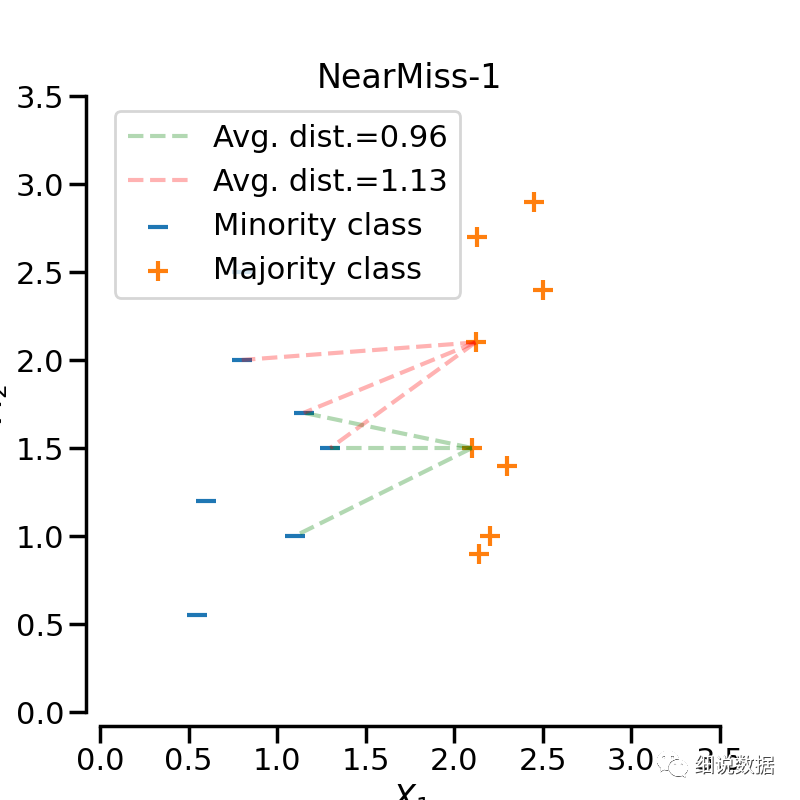
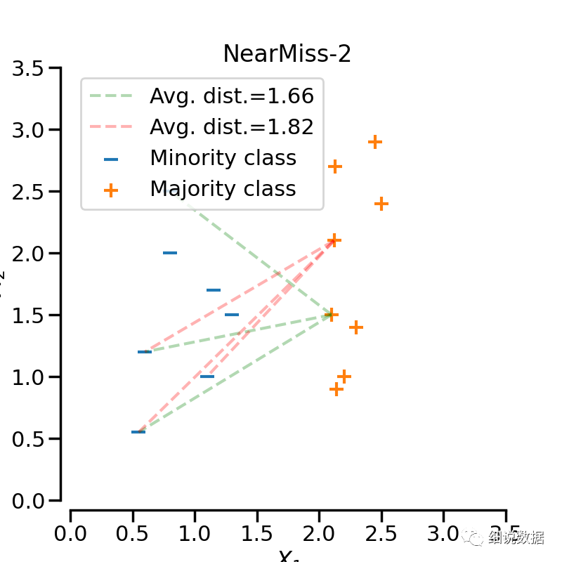
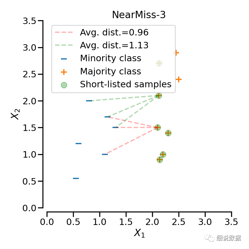
NearMiss

添加了一些启发式(heuristic)的规则来选择样本, 通过设定version参数来实现三种启发式的规则。假设正样本是需要下采样的(多数类样本), 负样本是少数类的样本。则：NearMiss-1: 选择离N个近邻的负样本的平均距离最小的正样本;NearMiss-2: 选择离N个负样本最远的平均距离最小的正样本;NearMiss-3: 是一个两段式的算法. 首先, 对于每一个负样本, 保留它们的M个近邻样本; 接着, 那些到N个近邻样本平均距离最大的正样本将被选择。

from imblearn.under_sampling import NearMiss
nm1 = NearMiss(version=1)
X_resampled_nm1, y_resampled = nm1.fit_resample(X, y)
print(sorted(Counter(y_resampled).items()))

结果：[(0, 64), (1, 64), (2, 64)]

清洁欠采样技术不允许指定每个类中的样本数量。事实上，每个算法都实现了一种启发式方法，可以清理数据集。

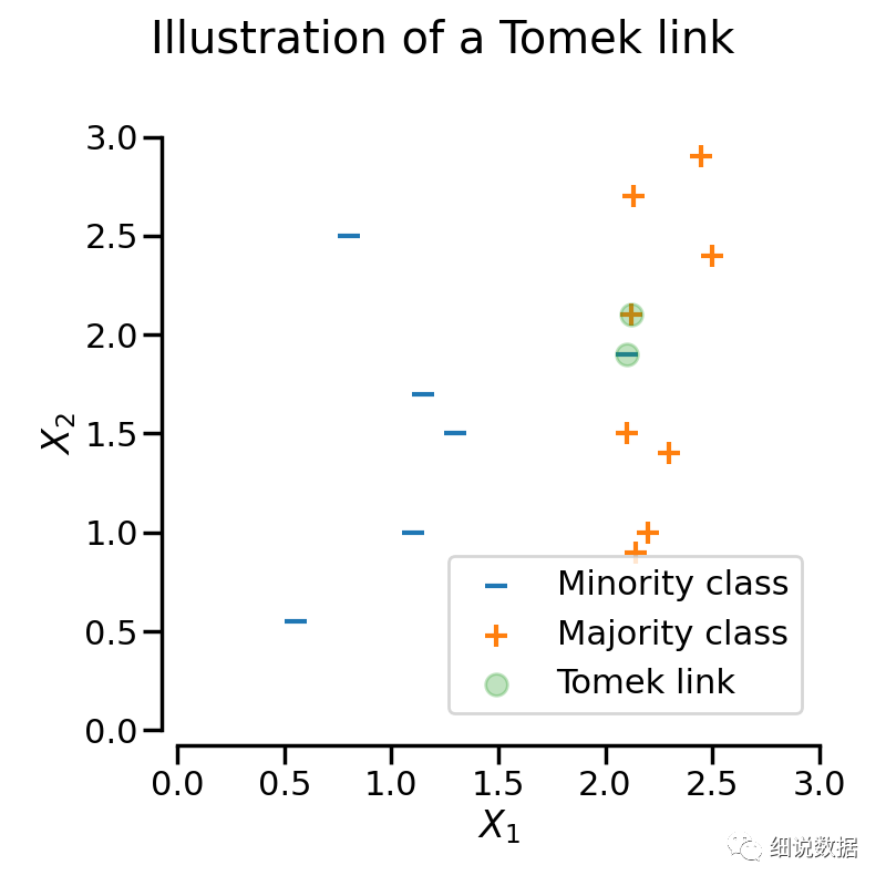
TomekLinks

样本x与样本y来自于不同的类别, 满足以下条件, 它们之间被称之为TomekLinks; 不存在另外一个样本z, 使得d(x,z) < d(x,y) 或者 d(y,z) < d(x,y)成立. 其中d(.)表示两个样本之间的距离, 也就是说两个样本之间互为近邻关系. 这个时候, 样本x或样本y很有可能是噪声数据, 或者两个样本在边界的位置附近.

from imblearn.under_sampling import TomekLinks 
tl = TomekLinks()
X_resampled, y_resampled = tl.fit_resample(X, y)
print(sorted(Counter(y_resampled).items()))

结果：[(0, 64), (1, 249), (2, 4654)]

EditedNearestNeighbours

这种方法应用最近邻算法来编辑(edit)数据集, 找出那些与邻居不太友好的样本然后移除. 对于每一个要进行下采样的样本, 那些不满足一些准则的样本将会被移除; 目前有两个选择标准：（i）多数（即 kind_sel='mode'）或（ii）所有（即kind_sel='all'）最近邻必须与检查的样本属于同一类以将其保留在数据集中。

from imblearn.under_sampling import EditedNearestNeighbours
enn = EditedNearestNeighbours()
X_resampled, y_resampled = enn.fit_resample(X, y)
print(sorted(Counter(y_resampled).items()))
enn_1 = EditedNearestNeighbours(kind_sel="mode")
X_resampled_1, y_resampled_1 = enn_1.fit_resample(X, y)
print(sorted(Counter(y_resampled_1).items()))

结果：[(0, 64), (1, 213), (2, 4568)]

[(0, 64), (1, 234), (2, 4666)]

RepeatedEditedNearestNeighbours

重复EditedNearestNeighbours多次

from imblearn.under_sampling import RepeatedEditedNearestNeighbours
renn = RepeatedEditedNearestNeighbours()
X_resampled, y_resampled = renn.fit_resample(X, y)
print(sorted(Counter(y_resampled).items()))

结果：[(0, 64), (1, 208), (2, 4551)]

ALLKNN

与RepeatedEditedNearestNeighbours算法不同的是, ALLKNN算法在进行每次迭代的时候, 最近邻的数量都在增加。

from imblearn.under_sampling import AllKNN
allknn = AllKNN()
X_resampled, y_resampled = allknn.fit_resample(X, y)
print(sorted(Counter(y_resampled).items()))

结果：[(0, 64), (1, 220), (2, 4601)]

CondensedNearestNeighbour

使用1近邻的方法来进行迭代, 来判断一个样本是应该保留还是剔除, 具体的实现步骤如下:

1)集合C: 所有的少数类样本;

2)选择一个多数类样本(需要下采样)加入集合C, 其他的这类样本放入集合S;

3)使用集合S训练一个1-NN的分类器, 对集合S中的样本进行分类;

4)将集合S中错分的样本加入集合C;

5)重复上述过程, 直到没有样本再加入到集合C。

from imblearn.under_sampling import CondensedNearestNeighbour
cnn = CondensedNearestNeighbour(random_state=0)
X_resampled, y_resampled = cnn.fit_resample(X, y)
print(sorted(Counter(y_resampled).items()))

结果：[(0, 64), (1, 24), (2, 115)]

OneSidedSelection

CondensedNearestNeighbour方法对噪音数据是很敏感的, 也容易加入噪音数据到集合C中。因此, OneSidedSelection 函数使用 TomekLinks 方法来剔除噪声数据(多数类样本)。

from imblearn.under_sampling import OneSidedSelection
oss = OneSidedSelection(random_state=0)
X_resampled, y_resampled = oss.fit_resample(X, y)
print(sorted(Counter(y_resampled).items()))

结果：[(0, 64), (1, 174), (2, 4404)]

NeighbourhoodCleaningRule

NeighbourhoodCleaningRule 算法主要关注如何清洗数据而不是筛选(considering)他们. 因此, 该算法将使用EditedNearestNeighbours和 3-NN分类器结果拒绝的样本之间的并集。

from imblearn.under_sampling import NeighbourhoodCleaningRule
ncr = NeighbourhoodCleaningRule()
X_resampled, y_resampled = ncr.fit_resample(X, y)
print(sorted(Counter(y_resampled).items()))

结果：[(0, 64), (1, 234), (2, 4666)]

InstanceHardnessThreshold

InstanceHardnessThreshold是一种特定算法，其中对数据训练分类器并删除概率较低的样本。有两个重要的参数。estimator将接受任何具有方法的 scikit-learn 分类器predict_proba。分类器训练使用交叉验证进行，参数cv可以设置要使用的折叠数。

from sklearn.linear_model import LogisticRegression
from imblearn.under_sampling import InstanceHardnessThreshold
iht = InstanceHardnessThreshold(random_state=0,
                                estimator=LogisticRegression(
                                solver='lbfgs', multi_class='auto'))
X_resampled, y_resampled = iht.fit_resample(X, y)
print(sorted(Counter(y_resampled).items()))

结果：[(0, 64), (1, 64), (2, 64)]

四、过采样和欠采样方法的结合

SMOTE算法的缺点是生成的少数类样本容易与周围的多数类样本产生重叠难以分类，而数据清洗技术恰好可以处理掉重叠样本，所以可以将二者结合起来形成一个pipeline，先过采样再进行数据清洗。主要的方法是 SMOTE + ENN 和 SMOTE + Tomek ，其中 SMOTE + ENN 通常能清除更多的重叠样本。

SMOTEENN

imblearn.combine.SMOTEENN(*, sampling_strategy='auto', 
random_state=None, smote=None, enn=None, n_jobs=None)

sampling_strategy：少数类中的样本数与多数类中的样本数的期望比率

random_state：随机数发生器

smote&enn：采样器对象

n_jobs：交叉验证循环期间使用的 CPU 内核数

from collections import Counter
from sklearn.datasets import make_classification
from imblearn.combine import SMOTEENN 
X, y = make_classification(n_classes=2, class_sep=2,
weights=[0.1, 0.9], n_informative=3, n_redundant=1, flip_y=0,
n_features=20, n_clusters_per_class=1, n_samples=1000, random_state=10)
print('Original dataset shape %s' % Counter(y))
sme = SMOTEENN(random_state=42)
X_res, y_res = sme.fit_resample(X, y)
print('Resampled dataset shape %s' % Counter(y_res))

结果：Original dataset shape Counter({1: 900, 0: 100})

Resampled dataset shape Counter({0: 900, 1: 881})

SMOTETomek

imblearn.combine.SMOTETomek(*, sampling_strategy='auto', 
random_state=None, smote=None, tomek=None, n_jobs=None)

sampling_strategy：少数类中的样本数与多数类中的样本数的期望比率

random_state：随机数发生器

smote&tomek：采样器对象

n_jobs：交叉验证循环期间使用的 CPU 内核数

from collections import Counter
from sklearn.datasets import make_classification
from imblearn.combine import SMOTETomek 
X, y = make_classification(n_classes=2, class_sep=2,
                           weights=[0.1, 0.9], n_informative=3, n_redundant=1, flip_y=0,
                           n_features=20, n_clusters_per_class=1, n_samples=1000, random_state=10)
print('Original dataset shape %s' % Counter(y))
smt = SMOTETomek(random_state=42)
X_res, y_res = smt.fit_resample(X, y)
print('Resampled dataset shape %s' % Counter(y_res))

结果：riginal dataset shape Counter({1: 900, 0: 100})
Resampled dataset shape Counter({0: 900, 1: 900})

总结：

参考文档：

https://blog.csdn.net/qq_31813549/article/details/79964973

https://imbalanced-learn.org/stable/references/generated/imblearn.over_sampling.ADASYN.html

https://www.cnblogs.com/massquantity/p/9382710.html

https://imbalanced-learn.org/stable/ensemble.html

https://blog.csdn.net/qq_24591139/article/details/100518532

数据库

文章转载自细说数据，如果涉嫌侵权，请发送邮件至：contact@modb.pro进行举报，并提供相关证据，一经查实，墨天轮将立刻删除相关内容。

失衡数据采样方法

fetch_datasets

scikit-learn 的 datasets 模块大规模数据集

SMOTEENN

SMOTETomek

评论