


1. What is time series?
什么是时间序列?
Some data change regularly with time. Time series is a sequence of data which are recorded in regular time interval. A time series can be in different frequency: hourly, daily, weekly, monthly,annually.
时间序列就是按照固定时间间隔的一串数字。这些数据的频率可以是每小时,每天,每周,每月,每年等等。
A good example of time series data are stock prices. Usually, we analyze stock prices using daily close prices, volumes,etc.
股票价格就是一串时间序列的数据。一般情况下,我们利用每日的收盘价、成交量等参数进行分析。
Sometimes, hedge funds analyze seconds or minute-wise time series stock prices for their high frequent trading. Therefore,you can choose the frequency of time series based on your purpose and data availability.
有些对冲基金为了做高频交易,需要用到秒或者分钟频率级别的数据。你可以根据你自身的需求以及是否能够获取到有关数据,选择时间序列的频率。
2. Why we need time seriesanalysis?
为什么要进行时间序列分析?
We need time series analysis because we want to know something about the future. From ancient time, people always want to have crystal balls tell them what will happen next. These crystal balls have been evolved to time series analysis and other machine learning models.
我们需要时间序列的原因在于我们想预测未来。从古至今,这个目标从未改变。过去的算命先生,现在有个好听的名字:数据科学家!只要人类存在,预测未来的工作总是有需求。即使你预测错了也没关系,没有人会投诉你,参见天气预报!
Sometimes, time series forecasting is very successful. We know that T mobile and citi bank near Columbia University will have more clients each August because of new students. Hot dog sales in Coney Island will rise every summer. In the long run, investing in stock market will receive a return close to 12%.
事实上,有些时间序列分析很成功。比方说我们知道学校附近的银行每天秋天会有很多新生来开户,夏天烧烤摊的生意会比冬天好。长期投资股市的收益率在12%左右。如果算命完全不正确,也就没有人会去算命了。
3. How to analyze financial timeseries with Python?
如何利用Python进行时间序列分析
The first step is to read financial time series into Python. How can we do that? I will use Tesla stock as an illustration.
我们首先要通过Python读入金融数据。怎么实现呢?我就用特斯拉的股票说明这个问题。
3.1 Read data from Yahoo!Finance
从雅虎金融读入数据
We import some Python libraries Pandas,Numpy, matplotlib.pyplot and pandas_datareader. pandas_datareader is the package that help us read Tesla stock price from Yahoo. If you don’t have pandas_datareader, you can install it in the command line using:
Pip install pandas_datareader
我们先引用一些程序包。Pandas_datareader是用来从Yahoo金融读数据的程序包。你要是没有装,可以打开命令提示符,然后用下列命令安装:
Pip install pandas_datareader
# Import some libraries
import pandas as pd
import numpy as np
import matplotlib.pyplot as plt
import pandas_datareader as pdr
Since we will analyze financial data, the next step is the set a start date and end date.
接下来是设定起始日期和结束日期:
# Set start and end date
start='2010-12-31'
end='2020-03-04'
Okay, we are ready to retrieve data from Yahoo!Finance. Just use following code:
好了,我们只需要用下面一行程序就可以从雅虎金融上提取特斯拉的数据。
TSLA = pdr.get_data_yahoo('Tsla',start=start, end=end)
If you want to retrieve other stocks like APPL, AMZN, GOOG, FB, just change the symbol. But for this time, I will keep using Tesla as my example.
你要是对别的股票感兴趣,可以换成它们的代码,比方说苹果,亚马逊,谷歌,脸书等等。我这里还是用特斯拉作为例子。
3.2 Check data with Pandas
用Pandas检验数据
A good habit is to check data using Pandas before you analyze them.
我们先用Pandas看看数据。
The time series dataset TSLA starts from 2010-12-31 and end at 2020-3-4. It has 2308 rows and 6 columns including High,Low, Volume, Adj Close. But there are two variables we can’t see.
时间序列数据集从2010年12月31日开始,到2020年3月4日结束。它有2308行以及最高价、最低价、成交量和复权后的价格。但是还有两个变量我们看不到。
TSLA.info
Out[83]:
<bound method DataFrame.info of High Low ... Volume Adj Close
Date ...
2010-12-31 27.250000 26.500000 ... 1417900 26.629999
2011-01-03 27.000000 25.900000 ... 1283000 26.620001
2011-01-04 26.950001 26.020000 ... 1187400 26.670000
2011-01-05 26.900000 26.190001 ... 1446700 26.830000
2011-01-06 28.000000 26.809999 ... 2061200 27.879999
2011-01-07 28.580000 27.900000 ... 2247900 28.240000
2011-01-10 28.680000 28.049999 ... 1342700 28.450001
2020-03-02 743.690002 686.669983 ... 20195000 743.619995
2020-03-03 806.979980 716.109985 ... 25784000 745.510010
2020-03-04 766.520020 724.729980 ... 15004800 749.500000
[2308 rows x 6 columns]>
But if we use head(), then we can see Ope nand Close
我们用head()就可以看到开盘价和收盘价。
TSLA.head()
Out[84]:
High Low Open Close Volume Adj Close
Date
2010-12-31 27.250000 26.500000 26.57 26.629999 1417900 26.629999
2011-01-03 27.000000 25.900000 26.84 26.620001 1283000 26.620001
2011-01-04 26.950001 26.020000 26.66 26.670000 1187400 26.670000
2011-01-05 26.900000 26.190001 26.48 26.830000 1446700 26.830000
2011-01-06 28.000000 26.809999 26.83 27.879999 2061200 27.879999
Shape() tells us similar information
Shape()函数得出的信息也差不多。
TSLA.shape
Out[85]: (2308, 6)
10 years ago, the little stock of tesla is only $26 per share.
10年前,特斯拉的股价只有26美元。
TSLA.Close.head()
Out[86]:
Date
2010-12-31 26.629999
2011-01-03 26.620001
2011-01-04 26.670000
2011-01-05 26.830000
2011-01-06 27.879999
Name: Close, dtype: float64
10 years later, one share of Tesla stock worth over $700. It rose 28.8 times!So if you spend $2,600 to buy 100 share of Tesla at the end of 2010, now theoretically speaking, you have $75,000. In this scenario, you’d better forget them after you bought them.
10年后,每股特斯拉的价格超过700美元。上涨超过28倍!如果你在2010年底买了100股特斯拉,花费2600美元,那么理论上讲现在你手里应该有大约7.5万美元!但是这只不过是理论上讲,能一直拿着不动的人很少很少。不信你可以试试!
TSLA.Close.tail()
Out[87]:
Date
2020-02-27 679.000000
2020-02-28 667.989990
2020-03-02 743.619995
2020-03-03 745.510010
2020-03-04 749.500000
Name: Close, dtype: float64
If we check the adjusted close price, we find they are the same as close price. This means Tesla did not give any dividend to shareholder and there is no stock split. However, if you are a disciple of value investment, you will not buy this stock because of dividend.Life is a box of chocolates!
特斯拉的复权价格和收盘价一样。这说明特斯拉这些年以来没有分红,也没有拆股。但如果你是一个价值投资者,你根本就不会买这样的股票,因为价值投资的原则之一是要买入分红的股票。
TSLA['Adj Close'].head()
Out[96]:
Date
2010-12-31 26.629999
2011-01-03 26.620001
2011-01-04 26.670000
2011-01-05 26.830000
2011-01-06 27.879999
Name: Adj Close, dtype: float64
TSLA['Adj Close'].tail()
Out[97]:
Date
2020-02-27 679.000000
2020-02-28 667.989990
2020-03-02 743.619995
2020-03-03 745.510010
2020-03-04 749.500000
Name: Adj Close, dtype: float64
In Pandas, you can select certain rows.
你还可以选点某些行的数据
TSLA.iloc[10:13]
Out[88]:
High Low Open Close Volume Adj Close
Date
2011-01-14 26.580000 25.610001 26.15 25.750000 1192000 25.750000
2011-01-18 25.639999 24.750000 25.48 25.639999 1621700 25.639999
2011-01-19 25.469999 23.750000 25.27 24.030001 2371500 24.030001
You can also do some statistical analysis for this. The minimum price is $21 and the maximum is $917. This means if you have crystal balls and buy at the bottom, sell at the peak, you can receive over 43 times return. Unfortunately, this is just a day dream for common people.
你还可以做一些统计分析。你会发现特斯拉股价的最低点是21美元,最高点是917美元。所以如果你能买到最低点,卖到最高点,那么你的收益超过43倍。不过对于普通人而言,这仅仅是个黄粱美梦!
TSLA['Close'].mean()
Out[91]: 201.01972715486895
TSLA['Close'].min()
Out[92]: 21.829999923706055
TSLA['Close'].max()
Out[93]: 917.4199829101562
We can also use describe() to make thisstatistics easier.
你可以用describe一步到位。
TSLA['Close'].describe()
Out[94]:
count 2308.000000
mean 201.019727
std 128.548347
min 21.830000
25% 47.615002
50% 219.450005
75% 277.867508
max 917.419983
Name: Close, dtype: float64
In Pandas, you can add variables to datasets. For example, you can add pct_return (daily percentage return) to the TSLA dataset using following code:
我们加入一个新变量,每日百分比收益率(也就是涨跌幅)
TSLA['pct_return'] =TSLA['Close'].pct_change()
Then you can see a new variable pct_return appears in TSLA.
然后这个变量就出现在数据集当中了。
TSLA.head()
Out[102]:
High Low Open ... Volume Adj Close pct_return
Date ...
2010-12-31 27.250000 26.500000 26.57 ... 1417900 26.629999 NaN
2011-01-03 27.000000 25.900000 26.84 ... 1283000 26.620001 -0.000375
2011-01-04 26.950001 26.020000 26.66 ... 1187400 26.670000 0.001878
2011-01-05 26.900000 26.190001 26.48 ... 1446700 26.830000 0.005999
2011-01-06 28.000000 26.809999 26.83 ... 2061200 27.879999 0.039135
[5 rows x 7 columns]
We can “describe” it. As the mean is 0.001967, we can say that if you hold Tesla in the past 10 years, you receive 0.2% everyday. But some days are good, some days are bad. In the best day, you have 24% in one single day! And you may also lose 20% in another day. C’est la vie!
TSLA['pct_return'].describe()
Out[103]:
count 2307.000000
mean 0.001967
std 0.032396
min -0.193274
25% -0.013804
50% 0.000871
75% 0.017642
max 0.243951
Name: pct_return, dtype: float64
We definitely want to know what date is ourlucky day! We have two days return higher than 18%. One day is 2013-5-9 (the VictoryDay!), 24.4%. Another day is 2020-2-3, 19.9%!
mask = (TSLA['pct_return'] > 0.18)
TSLA_high = TSLA[mask]
TSLA_high.head(10)
Out[106]:
High Low ... Adj Close pct_return
Date ...
2013-05-09 75.769997 63.689999 ... 69.400002 0.243951
2020-02-03 786.140015 673.520020 ... 780.000000 0.198949
[2 rows x 7 columns]
One ABNORMAL fact is that the log returns ofstock prices are normally distributed with mean of mu and standard deviation of sigma, which is denoted by N(mu, sigma).
And time series models as well as other financial models (such as the black Scholes model) always have the assumption of normal distribution. Thus, we’d better include daily log returns in our TSLA dataset. This can be done using following codes:
股票的对数收益率符合正态分布,我们把特斯拉每日对手收益率(log_return)也加入数据。这也是Pandas的基本功能。
TSLA['log_price'] = np.log(TSLA.Close)
TSLA['log_return'] =TSLA['log_price'].diff()
Now, we can see that there are pct_return,log_price and log_return in the dataset
现在我们的数据集里就有了log_return
TSLA.head()
Out[108]:
High Low Open ... pct_return log_price log_return
Date ...
2010-12-31 27.250000 26.500000 26.57 ... NaN 3.282038 NaN
2011-01-03 27.000000 25.900000 26.84 ... -0.000375 3.281663 -0.000376
2011-01-04 26.950001 26.020000 26.66 ... 0.001878 3.283539 0.001876
2011-01-05 26.900000 26.190001 26.48 ... 0.005999 3.289521 0.005981
2011-01-06 28.000000 26.809999 26.83 ... 0.039135 3.327910 0.038389
3.3 Test for normality
正态分布检验
Let’s use Shapiro-Wilk test to see if Tesla’s daily log returns are normally distributed. For Shapiro-Wilk test
H0: dataare normally distributed
Ha: dataare not normally distributed
Sine the p-value is much less than alpha,we reject the null hypothesis.
我们用Shapiro-Wilk test检验特斯拉每日对数收益率是否为正态分布。由于p指太小,所以特斯拉每日对数收益率并非正态分布。太不幸了!
# normality test
from scipy.stats import shapiro
stat, p =shapiro(TSLA['log_return'].dropna())
print('Statistics=%.3f, p=%.3f' % (stat,p))
# interpret
alpha = 0.05
if p > alpha:
print('Samplelooks Gaussian (fail to reject H0)')
else:
print('Sampledoes not look Gaussian (reject H0)')
Statistics=0.927, p=0.000
Sample does not look Gaussian (reject H0)
3.4 Visualiztion
可视化
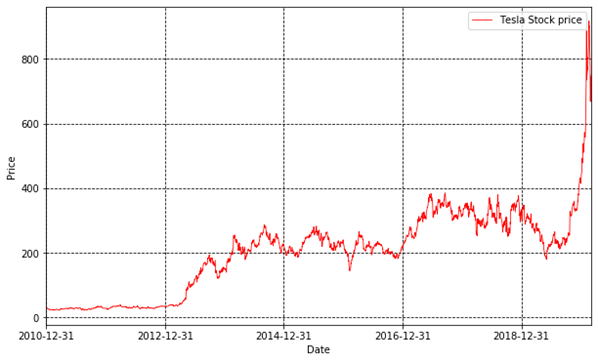
Finally, we need to visualize our data. The first important thing is to plot Tesla’s stock price:
首先,我们画出特斯拉的股票价格:
importmatplotlib.dates as mdate
plt.plot(TSLA.Close,'r',linewidth=0.8,markersize=12,label='Tesla Stock price')
plt.legend()
plt.xlabel('Date')
plt.ylabel('Price')
ax = plt.gca()
ax.xaxis.set_major_formatter(mdate.DateFormatter('%Y-%m-%d'))
plt.xticks(pd.date_range(start,end,freq='2y'))
plt.yticks(fontsize=10,rotation=0)
plt.xlim(start,end)
plt.grid(c='k',linestyle='--')
plt.rcParams['figure.figsize']= (10.0, 6.0)
plt.show()
Fig.1
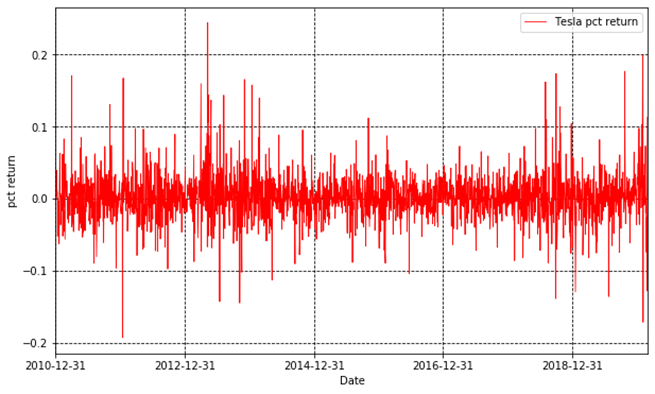
Then, we plot the daily percentage returns.
接下来,我们画出每日涨跌幅。
plt.plot(TSLA.pct_return,'r',linewidth=0.8,markersize=12,label='Tesla pct return')
plt.legend()
plt.xlabel('Date')
plt.ylabel('pct return')
ax = plt.gca()
ax.xaxis.set_major_formatter(mdate.DateFormatter('%Y-%m-%d'))
plt.xticks(pd.date_range(start,end,freq='2y'))
plt.yticks(fontsize=10,rotation=0)
plt.xlim(start,end)
plt.grid(c='k',linestyle='--')
plt.rcParams['figure.figsize'] = (10.0, 6.0)
plt.show()
Fig.2
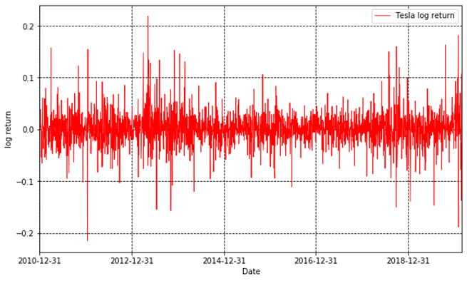
At last, we plot the log returns.
最后画出对数收益。
plt.plot(TSLA.log_return,'r',linewidth=0.8,markersize=12,label='Tesla log return')
plt.legend()
plt.xlabel('Date')
plt.ylabel('log return')
ax = plt.gca()
ax.xaxis.set_major_formatter(mdate.DateFormatter('%Y-%m-%d'))
plt.xticks(pd.date_range(start,end,freq='2y'))
plt.yticks(fontsize=10,rotation=0)
plt.xlim(start,end)
plt.grid(c='k',linestyle='--')
plt.rcParams['figure.figsize'] = (10.0,6.0)
plt.show()
Fig.3
Python十二钗之Scikit-learn :特朗普的就职演说有何不同?
Python十二钗之SciPy:早知有SciPy,何必用美拍?
Python十二钗之Matplotlib:画图原来如此简单!
