06【C-8m s】High-Speed Autonomous Racing Using.pdf

Zixin Huo

7页

0次

2023-10-19

25墨值下载

IEEE ROBOTICS AND AUTOMATION LETTERS, VOL. 8, NO. 9, SEPTEMBER 2023 5353

High-Speed Autonomous Racing Using

Trajectory-Aided Deep Reinforcement Learning

Benjamin David Evans , Herman Arnold Engelbrecht , Senior Member, IEEE,

and Hendrik Willem Jordaan

, Senior Member, IEEE

Abstract—The classical method of autonomous racing uses real-

time localisation to follow a precalculated optimal trajectory. In

contrast, end-to-end deep reinforcement learning (DRL) can train

agents to race using only raw LiDAR scans. While classical meth-

ods prioritise optimization for high-performance racing, DRL ap-

proaches have focused on low-performance contexts with little

consideration of the speed proﬁle. This work addresses the prob-

lem of using end-to-end DRL agents for high-speed autonomous

racing. We present trajectory-aided learning (TAL) that trains

DRL agents for high-performance racing by incorporating the

optimal trajectory (racing line) into the learning formulation. Our

method is evaluated using the TD3 algorithm on four maps in the

open-source F1Tenth simulator. The results demonstrate that our

method achieves a signiﬁcantly higher lap completion rate at high

speeds compared to the baseline. This is due to TAL training the

agent to select a feasible speed proﬁle of slowing down in the corners

and roughly tracking the optimal trajectory.

Index Terms—Deep learning methods, machine learning for

robot control, reinforcement learning.

I. INTRODUCTION

UTONOMOUS racing is a useful testbed for high-

performance autonomous algorithms due to the nature of

competition and the easy-to-measure performance metric of lap

time [1]. The aim of autonomous racing is to use onboard sensors

to calculate control references that move the vehicle around the

track as quickly as possible. Good racing performance operates

the vehicle on the edge of its physical limits between going too

slowly, which is poor racing behaviour, and going too fast, which

results in the vehicle crashing.

The classical robotics approach uses control systems that

depend on explicit state estimation to calculate references for the

robot’s actuators [2]. Classical racing systems use a localisation

algorithm to determine the vehicle’s pose on a map, which a

path follower uses to track an optimal trajectory [3]. Methods

requiring explicit state representation (localisation) are limited

by requiring a map of the track and being inﬂexible to environ-

mental changes [4].

Manuscript received 26 January 2023; accepted 2 July 2023. Date of pub-

lication 13 July 2023; date of current version 19 July 2023. This letter was

recommended for publication by Associate Editor H. Seok Ahn and Editor

A. Faust upon evaluation of the reviewers’ comments. (Corresponding author:

Benjamin David Evans.)

The authors are with the Department of Electrical and Electronic Engi-

neering, Stellenbosch University, Stellenbosch 7600, South Africa (e-mail:

bdevans@sun.ac.za; hebrect@sun.ac.za; wjordaan@sun.ac.za).

Digital Object Identiﬁer 10.1109/LRA.2023.3295252

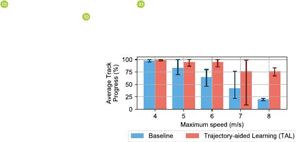
Fig. 1. Our method achieves signiﬁcantly higher average progress around the

track at high speeds than the baseline.

In contrast to classical methods, deep learning agents use

a neural network to map raw sensor data (LiDAR scans) di-

rectly to control commands without requiring explicit state

estimation [5]. Deep reinforcement learning (DRL) trains neural

networks from experience to select actions that maximise a

reward signal [6]. Previous DRL approaches have presented

end-to-end solutions for F1Tenth racing but have been limited to

low speeds [7], [8], and have lacked consideration of the speed

proﬁle [9].

This letter approaches the problem of how to train DRL

agents for high-speed racing using only a LiDAR scan as in-

put. We provide insights on learning formulations for training

DRL agents for high-performance control through the following

contributions:

1) Present trajectory-aided learning (TAL), which uses an

optimal trajectory to train DRL agents for high-speed

racing using raw LiDAR scans as input.

2) Demonstrate that TAL improves the completion rate of

DRL agents at high speeds compared to the baseline

learning formulation, as shown in Fig. 1.

3) Demonstrate that TAL agents select speed proﬁles sim-

ilar to the optimal trajectory and outperform related ap-

proaches in the literature.

II. L

ITERATURE STUDY

We study methods of autonomous racing in the categories of

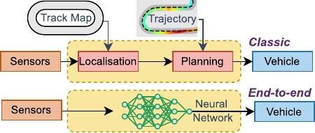
classical methods and end-to-end learning. Fig. 2 shows how the

classical racing pipeline uses a localisation module to enable a

planner to track a precomputed optimal trajectory, and end-to-

end learning replaces the entire pipeline with a neural network-

based agent.

See https://www.ieee.org/publications/rights/index.html for more information.

Authorized licensed use limited to: Shenzhen Institute of Advanced Technology CAS. Downloaded on October 11,2023 at 14:34:47 UTC from IEEE Xplore. Restrictions apply.

5354 IEEE ROBOTICS AND AUTOMATION LETTERS, VOL. 8, NO. 9, SEPTEMBER 2023

Fig. 2. Classical racing stack using localisation and planning modules, and

end-to-end racing using a neural network without state estimation.

A. Classical Racing

The classical racing method calculates an optimal trajectory

and then uses a path-following algorithm to track it [1]. Trajec-

tory optimisation techniques calculate a set of waypoints (posi-

tions with a s peed reference) on a track that, when followed, lead

the vehicle to complete a lap in the shortest time possible [3].A

path-following algorithm tracks the trajectory using the vehicle’s

pose as calculated by a localisation algorithm.

Localisation: Localisation approaches for autonomous racing

depend on the sensors and computation available. Full-sized

racing cars are often equipped with GPS (GNSS), LiDAR,

radar, cameras, IMUs, and powerful computers that can fuse

these measurements in real-time [10]. Classical F1Tenth racing

approaches have used a particle ﬁlter that takes a LiDAR scan

and a map of the track to estimate the vehicle’s pose [2], [4],

[11]. Localisation methods are inherently limited by requiring a

race track map and, thus, are inﬂexible to unmapped tracks.

Classical Path-Following: Model-predictive controllers

(MPC) and pure pursuit path-followers have been used for

trajectory tracking [1]. MPC planners calculate optimal con-

trol commands in a receding horizon manner [12] and have

demonstrated high-performance results racing F1Tenth vehicles

at speeds of up to 7 m/s [2]. The pure pursuit algorithm uses

a geometric model to calculate a steering angle to follow the

optimal trajectory [13], and has been used to race at speeds of

7m/s[11] and over 8 m/s [14].

Learning-based Path-following: Classical path-following al-

gorithms have been replaced by neural networks, aiming to

improve computational efﬁciency (compared to MPC) [12],

[15] and performance in difﬁcult-to-model conditions such as

drifting [16]. Including upcoming trajectory points in the state

vector (as opposed to only centerline points [15]) has shown to

improve racing performance [17], [18]. This shows demonstrates

that using the optimal trajectory results in high-performance

racing.

While classical and learning-based path-following methods

have produced high-performance results, they are inherently

limited by requiring the vehicle’s location on the map.

B. End-to-end Learning

In contrast to classical methods that use a perception, planning

and control pipeline, end-to-end methods use a neural network

to map raw sensory data to control references [9]. While some

approaches have used camera images [19], the dominant input

has been LiDAR scans [7], [9], [20].

Autonomous Driving: End-to-end learning agents can use a

subset of beams from a LiDAR scan to output steering references

that control a vehicle travelling at constant speed [7]. While

imitation learning (IL) has been used to train agents to copy an

expert policy [21], deep reinforcement learning, has shown bet-

ter results, with higher lap completion rates [7]. DRL algorithms

train agents in an environment (simulation [7] or real-world

system [20] ), where at each timestep, the agent receives a state,

selects an action and then receives a reward. DRL approaches to

driving F1Tenth vehicles have considered low, constant speeds

of 1.5 m/s [7], [22],2m/s[20], and 2.4 m/s [8]. While indicating

that DRL agents can control a vehicle, these methods neglect the

central racing challenge of speed selection.

Autonomous Racing: Using model-free end-to-end DRL

agents to select speed and steering commands for autonomous

racing is a difﬁcult problem [23], [24]. In response, Brunnbauer

et al. [23] turned to model-based learning and Zhang et al. [24]

incorporated an artiﬁcial potential ﬁeld planner in the learning

to simplify t he learning problem. Both [23] and [24] show that

their agents regularly crash while using top speeds of only

5 m/s, demonstrating the difﬁculty of learning for high-speed

autonomous racing. Bosello et al. [9] use a model-free DRL

algorithm (DQN) for F1Tenth racing at speeds of up to 5 m/s,

but provide no detail on the speed proﬁle, trajectory or crash

rate.

Summary: Classical racing methods have produced high-

performance racing behaviour using high maximum speeds but

are limited by requiring localisation. In contrast, end-to-end

DRL agents are successful in controlling vehicles at low speeds

using only the LiDAR scan as input. While some methods have

approached speed selection using DRL agents, there has been

little study on the speed proﬁles selected, and the highest speed

used is 5 m/s, which is signiﬁcantly less than classical methods of

8 m/s. This letter targets the gap in developing high-performance

racing solutions for steering and speed control in autonomous

race cars.

III. M

ETHODOLOGY

A. Reinforcement Learning Preliminary

Deep reinforcement learning (DRL) trains autonomous

agents, consisting of deep neural networks, to maximise a reward

signal from experience [6]. Reinforcement learning problems

are modelled as Markov Decision Processes (MDPs), where the

agent receives a state s from the environment and selects an

action a. After each action has been executed, the environment

returns a reward r indicating how good or bad the action was

and a new state s



This work considers deep-deterministic-policy-gradient

(DDPG) algorithms since we work with a continuous action

space [25]. DDPG algorithms maintain two neural networks, an

actor μ that maps a state to an action and a critic Q that evaluates

the action-value function. A pair of networks are maintained for

the actor and the critic; the model networks are used to select

actions, and target networks calculate the targets μ



and Q