MLog: Towards Declarative In-Database Machine Learning.pdf

盖国强

130

4页

0次

2024-01-27

5墨值下载

MLog: Towards Declarative In-Database Machine Learning

Xupeng Li

†

Bin Cui

†

Yiru Chen

†

Wentao Wu

∗

Ce Zhang

‡

†

School of EECS & Key Laboratory of High Conﬁdence Software Technologies (MOE),

Peking University {lixupeng, bin.cui, chen1ru}@pku.edu.cn

∗

Microsoft Research, Redmond wentao.wu@microsoft.com

‡

ETH Zurich ce.zhang@inf.ethz.ch

ABSTRACT

We demonstrate MLOG, a high-level language that integrates ma-

chine learning into data management systems. Unlike existing ma-

chine learning frameworks (e.g., TensorFlow, Theano, and Caffe),

MLOG is declarative, in the sense that the system manages all

data movement, data persistency, and machine-learning related op-

timizations (such as data batching) automatically. Our interactive

demonstration will show audience how this is achieved based on

the novel notion of tensoral views (TViews), which are similar

to relational views but operate over tensors with linear algebra.

With MLOG, users can succinctly specify not only simple mod-

els such as SVM (in just two lines), but also sophisticated deep

learning models that are not supported by existing in-database an-

alytics systems (e.g., MADlib, PAL, and SciDB), as a series of

cascaded TViews. Given the declarative nature of MLOG, we fur-

ther demonstrate how query/program optimization techniques can

be leveraged to translate MLOG programs into native TensorFlow

programs. The performance of the automatically generated Tensor-

Flow programs is comparable to that of hand-optimized ones.

1. INTRODUCTION

As of 2016, it is no longer easy to argue against the importance of

supporting machine learning in data systems. In fact, most modern

data management systems support certain types of machine learn-

ing and analytics. Notable examples include MADlib, SAP PAL,

MLlib, and SciDB. These systems are tightly integrated into the re-

lational data model, but treat machine learning as black-box func-

tions over relations/tensors. This results in a lack of ﬂexibility in

the types of machine learning models that can be supported.

On the other hand, machine learning systems such as Tensor-

Flow, Theano, and Caffe are made much more expressive and ﬂex-

ible by exposing the mathematical structure of machine learning

models to the users. However, these systems do not have a declar-

ative data management layer — it is the user’s responsibility to

deal with such tedious and often error-prone tasks as data loading,

movement, and batching in these systems.

Given these limitations, it is not surprising that higher-level ma-

chine learning libraries such as Keras have become increasingly

This work is licensed under the Creative Commons Attribution-

NonCommercial-NoDerivatives 4.0 International License. To view a copy

of this license, visit http://creativecommons.org/licenses/by-nc-nd/4.0/. For

any use beyond those covered by this license, obtain permission by emailing

info@vldb.org.

Data Model Integration

Query Language Integration

SciDB

MADlib

SAP PAL

Our

Goal

Relational Model Tensor Model

Relational

Queries

Blackbox

ML Functions

Linear Algebra

Primitives

Mathematical

Optimization

Queries

Figure 1: Schematic Comparison with Existing Systems.

popular. Given the data as a numpy array, Keras is fully declar-

ative and users only need to specify the logical dependencies be-

tween these arrays, rather than specifying how to solve the result-

ing machine learning model. However, a system like Keras does not

provide data management for these numpy arrays and it is still the

user’s responsibility to take care of low-level programming details

such as whether these arrays ﬁt in memory, or textbook database

functionality such as reuse computation across runs or “time travel”

through training snapshots. Moreover, Keras cannot be integrated

into the standard relational database ecosystem that hosts most of

the enterprise data.

In this paper, we demonstrate MLOG, a system that aims for

marrying Keras-like declarative machine learning to SciDB-like

declarative data management. In MLOG, we build upon a standard

data model similar to SciDB, to avoid neglecting and reinventing

decades of study of data management. Our approach is to extend

the query language over the SciDB data model to allow users to

specify machine learning models in a way similar to traditional re-

lational views and relational queries. Speciﬁcally, we demonstrate

the following three main respects of MLOG:

(Declarative Query Language) We demonstrate a novel query

language based on tensoral views that has formal seman-

tics compatible with existing relational-style data models and

query languages. We also demonstrate how this language al-

lows users to specify a range of machine learning models,

including deep neural networks, very succinctly.

(Automated Query Optimization) We demonstrate how to auto-

matically compile MLOG programs into native TensorFlow

programs using textbook static analysis techniques.

(Performance) We demonstrate the performance of automatically

generated TensorFlow programs on a range of machine learn-

ing tasks. We show that the performance of these programs

is often comparable to (up to 2× slower than) manually op-

timized TensorFlow programs.

Limitations. As a preliminary demonstration of our system, the

current version of MLOG has the following limitations. First, our

ultimate goal is to fully integrate MLOG into SciDB and Post-

1933

(UFEAT, MFEAT) <- \argmin_{UFEAT, MFEAT} LOSS

LOSS <- \sum_{i,j} (R_{i,j} - RATINGS_{i,j})^2;

R_{i,j} <- UFEAT_{i,-} * MFEAT_{j,-}’;

create tensor MFEAT (movie, fid 1:100) -> feature;

create tensor UFEAT (user, fid 1:100) -> feature;

create tensor RATINGS(user, movie) -> rating;

Schema

View

Query

(1) MLog Program (2) Datalog Program

LOSS(v) :- R(i,j,v1), RATINGS(i,j,v2), v=op(i,j,v1,v2)

R(i,j,v) :- UFEAT(i,j1,v1), MFEAT(j,j2,v2), v=op(j1,v1,j2,v2)

(3.2) Executable Program

“Datalog-ify”

(3.1) Human-readable Math

Static Analysis & Optimiser

Y_{s,t} <- \sigma(Wy*H_{s,t,-});

H_{s,t,-} <- \sigma(Wh*X_{s,t,-} + Uh*H_{s,t-1,-});

create tensor Y(sent, word)-> feat;

create tensor H(sent, word, fid 1:100)-> feat;

create tensor X(sent, word, fid 1:100)-> feat;

Schema

View

(1) MLog Program (2) Datalog Program

H(s,t,v) :- Wh(w),X(s,t,v1),Uh(u),H(s,t-1,v2), v=op(w,v1,u,v2)

H(s,t,v) :- sent(s), t=0, v=0

(3.2) Executable Program

“Datalog-ify”

(3.1) Human-readable Math

Static Analysis & Optimiser

H_{s,0,-} <- 0;

create tensor ANS(sent, word)-> feat;

LOSS <- \sum_{i,j} (Y_{s,t} - ANS_{s,t})^2;

(Wh, Wy, Uh) <- \argmin_{Wh, Wy, Uh} LOSS

Query

create tensor Uh(fid 1:100, fid 1:100)-> feat;

create tensor Wh(fid 1:100, fid 1:100)-> feat;

create tensor Wy(fid 1:100)-> feat;

LOSS(v) :- Y(s,t,v1), ANS(s,t,v2), v=op(s,t,v1,v2)

Y(s,t,v) :- Wy(w),H(s,t,v1), v=op(w,v1)

(a)

(b)

(c)

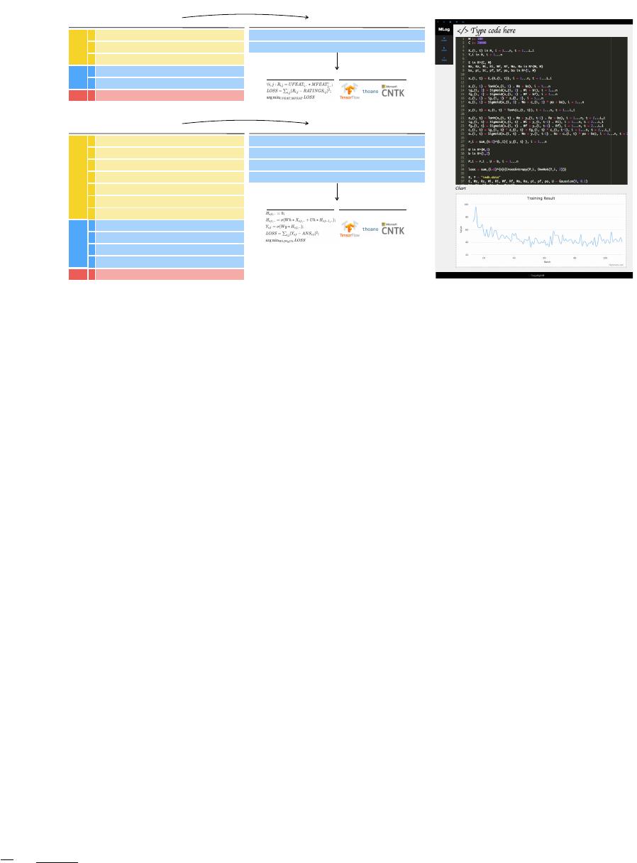
Figure 2: MLOG Examples for (a) Matrix Factorization and (b) Recurrent Neural Network. (c) User Interface of MLOG.

greSQL such that it runs on the same data representation and users

can use a mix of MLOG and SQL statements. Although our formal

model provides a principled way for this integration, this function-

ality has not been implemented yet. In this demonstration, we focus

on the machine learning component and leave the full integration

as future work. Second, the current MLOG optimizer does not con-

duct special optimizations for sparse tensors. (In fact, it does not

even know the sparsity of the tensor.) Sparse tensor optimization is

important for a range of machine learning tasks, and we will sup-

port it in the near future. Third, the current performance of MLOG

can still be up to 2× slower than hand-optimized TensorFlow pro-

grams. It is our ongoing work to add more optimization rules into

the optimizer and to build our system on a more ﬂexible backend,

e.g. Angel [6, 5]. Despite these limitations, we believe the current

MLOG prototype can stimulate discussions with the audience about

the ongoing trend of supporting machine learning in data manage-

ment systems.

Reproducibility and Public Release. The online demo will

be up before the conference. For now, all MLOG programs, hand-

crafted TensorFlow programs, and automatically generated Tensor-

Flow programs are available at github.com/DS3Lab/MLog.

2. THE MLOG LANGUAGE

In this section, we present basics for the audience to understand

the syntax and semantics of the MLOG language.

2.1 Data Model

The data model of MLOG is based on tensors–all data in MLOG

are tensors and all operations are a subset of linear algebra over

tensors. In MLOG, the tensors are closely related to the relational

model; in fact, logically, a tensor is deﬁned as a special type of re-

lation. Let T be a tensor of dimension dim(T ) and let the index of

each dimension j range from {1, ..., dom(T, j)}. Logically, each

tensor T corresponds to a relation RJT K with dim(T )+1 attributes

, ..., a

dim(T )

, v), where the domain of a

is {1, ..., dom(T, j)}

and the domain of v is the real space R. Given a tensor T ,

RJT K = {(a

, ..., a

dim(T )

, v)|T [a

, ..., a

dim(T )

] = v},

where T [a

, ..., a

dim(T )

] is the tensor indexing operation that gets

the value at location (a

, ..., a

dim(T )

Algebra over Tensors. We deﬁne a simple algebra over tensors

and deﬁne its semantics with respect to RJ−K, which allows us to

tightly integrate operation over tensors into a relational database

and Spark with uniﬁed semantics. This algebra is very similar to

DataCube with extensions that support linear algebra operations.

We illustrate it with two example operators:

1. Slicing σ. The operator σ

¯x

(T ) subselects part of the input

tensor and produces a new “subtensor.” The j-th element

of ¯x, i.e., ¯x

∈ 2

{1,...,dom(T,j)}

, deﬁnes the subselection

on dimension j. The semantic of this operator is deﬁned as

RJσ

¯x

(T )K =

{(a

, ..., a

dim(T )

, v)|a

∈ ¯x

∧(a

, ..., a

dim(T )

, v) ∈ RJT K}.

2. Linear algebra operators op. We support a range of linear

algebra operators, including matrix multiplication and con-

volution. These operators all have the form op(T

, T

) and

their semantics are deﬁned as RJop(T

, T

)K =

{(a

, ..., a

dim(T )

, v)|op(T

, T

)[a

, ..., a

dim(T )

] = v}.

2.2 MLog Program

An MLOG program Π consists of a set of TRules (tensoral rules).

TRule. Each TRule is of the form

T (¯x) : −op (T

(¯x

), ..., T

(¯x

)) ,

where n ≥ 0. Similar to Datalog, we call T (¯x) the head of the

rule, and T

(¯x

), ..., T

(¯x

) the body of the rule. We call op the

operator of the rule. Each ¯x

and ¯x speciﬁes a subselection that

can be used by the slicing operator σ. To simplify notation, we use

“−” to donate the whole domain of each dimension–for example,

if ¯x = (5, −), σ

¯x

(T ) returns a subtensor that contains the entire

ﬁfth row of T . We deﬁne the forward evaluation of a TRule as the

process that takes as input the current instances of the body tensors,

and outputs an assignment for the head tensor by evaluating op.

Semantics. Similar to Datalog programs, we can deﬁne ﬁxed-

point semantics for MLOG programs. Let I be a data instance that

contains the current result of each tensor. We deﬁne the immediate

consequence of program Π on I as S

(I), which contains I and

all forward evaluation results for each TRule. The semantic of an

MLOG program is the least ﬁxed point of S

(I), i.e., S

∞

(I) = I.

1934