Learning Autoregressive Model in LSM-Tree based Store.pdf

Apache IoTDB

11页

0次

2024-03-27

100墨值下载

Learning Autoregressive Model in LSM-Tree based Store

Yunxiang Su

Tsinghua University

Beijing, China

suyx21@mails.tsinghua.edu.cn

Wenxuan Ma

Tsinghua University

Beijing, China

mwx22@mails.tsinghua.edu.cn

Shaoxu Song

BNRist, Tsinghua University

Beijing, China

sxsong@tsinghua.edu.cn

ABSTRACT

Database-native machine learning operators are highly desired for

ecient I/O and computation costs. While most existing machine

learning algorithms assume the time series data fully available and

readily ordered by timestamps, it is not the case in practice. Com-

modity time series databases store the data in pages with possibly

overlapping time ranges, known as LSM-Tree based storage. Data

points in a page could be incomplete, owing to either missing values

or out-of-order arrivals, which may be inserted by the imputed or

delayed points in the following pages. Likewise, data points in a

page could also be updated by others in another page, for dirty data

repairing or re-transmission. A straightforward idea is thus to rst

merge and order the data points by timestamps, and then apply the

existing learning algorithms. It is not only costly in I/O but also pre-

vents pre-computation of model learning. In this paper, we propose

to oine learn the AR models locally in each page on incomplete

data, and online aggregate the stored models in dierent pages with

the consideration of the aforesaid inserted and updated data points.

Remarkably, the proposed method has been deployed and included

as a function in an open source time series database, Apache IoTDB.

Extensive experiments in the system demonstrate that our proposal

LSMAR shows up to one order-of-magnitude improvement in learn-

ing time cost. It needs only about 10s of milliseconds for learning

over 1 million data points.

CCS CONCEPTS

• Information systems

→

Query operators; • Computing method-

ologies → Machine learning.

KEYWORDS

Autoregressive models, LSM store, in-database operators

ACM Reference Format:

Yunxiang Su, Wenxuan Ma, and Shaoxu Song. 2023. Learning Autoregressive

Model in LSM-Tree based Store. In Proceedings of the 29th ACM SIGKDD

Conference on Knowledge Discovery and Data Mining (KDD ’23), August

6–10, 2023, Long Beach, CA, USA. ACM, New York, NY, USA, 11 pages.

https://doi.org/10.1145/3580305.3599405

1 INTRODUCTION

IoT data are often collected in a preset frequency, e.g., in every

second, leading to time series with regular intervals. However,

the data arrivals are often out-of-order, owing to various network

This work is licensed under a Creative Commons Attribution

International 4.0 License.

KDD ’23, August 6–10, 2023, Long Beach, CA, USA

ACM ISBN 979-8-4007-0103-0/23/08.

https://doi.org/10.1145/3580305.3599405

Page 1 Page 2

320

327

Value

Imputation Repair

Delay

Re-transmission

Time

Version

320

327

Value

ଵ

ݔො

ଶ

ଷ

଺

ݔො

଻

଼

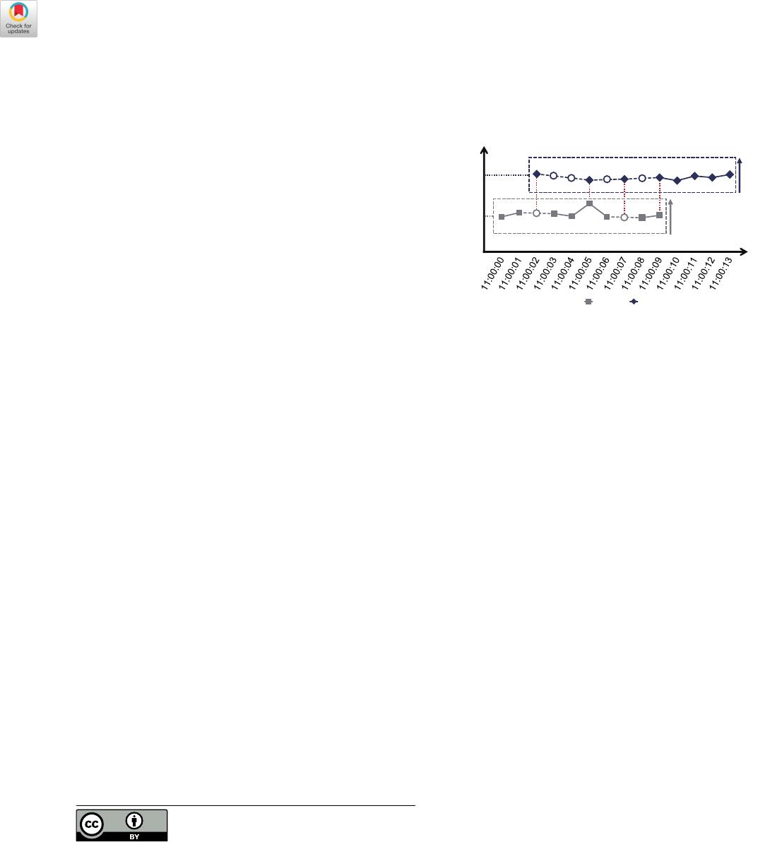
Figure 1: Example of imputed, repaired, delayed and re-

transmitted data in LSM-Tree store for learning AR models

delays in the IoT scenarios [

]. Moreover, some points could

be missing and inserted back by data imputation program [

Furthermore, dirty values are also detected and updated later by

requesting point re-transmission or data repairing program [26].

To handle the aforesaid out-of-order arrival, point insertion for

imputation, value update for repairing and so on [

], most com-

modity time series databases, such Apache IoTDB [

], employ a

Log-Structured Merge-Tree (LSM-Tree) [

] based storage. As illus-

trated in Figure 1, data points are batched in disk pages referring

to their arrivals. Some points such as the one at time 11:00:07 are

delayed and batched with other data points in page 2. The cor-

responding position in page 1 is thus denoted by a hollow circle.

Likewise, the missing point at time 11:00:02 is imputed, again in

page 2. Moreover, the point at time 11:00:05 with dirty value in

page 1 is repaired later by the one at the same time in page 2, while

the point at time 11:00:09 is updated by data re-transmission.

To learn models over the time series scattered in dierent pages

with possibly overlapping time ranges, a straightforward idea is to

rst load the data in disk pages to memory. Then, they are merged

by inserting the delayed or imputed points, and updating the re-

transmitted or repaired points. Existing learning algorithms [

] can

thus be applied over the merged time series ordered by time. It

is obviously inecient in I/O cost to read many stale data points

and merge them online. Moreover, the insertion and update of data

points also prevent directly utilizing the pre-computed models in

individual page when it is written to disk.

In this paper, we propose to design ecient schemes for online

aggregating the pre-computed models locally in each page. The

autoregressive (AR) is considered, since it is simple enough to learn

during the ush of the corresponding page to disk in database

ingestion. As illustrated in Figure 1, the model is pre-trained over

the incomplete time series in page 1 and stored. Intuitively, when

2061

KDD ’23, August 6–10, 2023, Long Beach, CA, USA Yunxiang Su, Wenxuan Ma, and Shaoxu Song

Table 1: Notations

Symbol Description

x time series of n = ∥x∥ data points

ℎ

, x

ℎ

) time and value of ℎ-th data point in x

p the autoregressive model order

𝛾

𝑖

the 𝑖-th order auto-covariances validity of time series x

𝜙

𝑖

the 𝑖-th autoregressive model coecient

new data points appear, e.g., in page 2, the pre-computed models

could be ne-tuned rather than learning from scratch.

Our major contributions in this study are as follows.

(1) We devise the learning process of models in a single page in

Section 3, including learning models with imputation, and updating

models with modied points.

(2) We propose the ecient aggregation of models learned in

dierent pages, with the consideration of inserted and updated

values, in Section 4. For pages with various cases, i.e., adjacent,

disjoint and overlapped in time ranges, we derive the corresponding

model aggregation strategies, respectively. The theoretical results

in Propositions 4.1, 4.3, 4.5 and 4.7 guarantee the correctness of

model aggregation, i.e., equivalent to the baseline of learning over

the merged time series.

(3) We present the algorithm for learning models on time series

scattered in dierent pages in Section 5. The complexity analysis

illustrates that our proposal is more ecient than the baseline of

learning from scratch over the online merged time series. Moreover,

we provide the details about system deployment, as a function

in Apache IoTDB [

], an open-source time series database. The

document is available in the product website [

], and the code is

included in the product repository by system developers [1].

(4) We conduct extensive experiments for evaluation in Section

6. Our proposal LSMAR shows up to one order-of-magnitude im-

provement in learning time cost, compared to the aforesaid baseline

of online merging data and learning from scratch. It needs only

about tens of milliseconds for learning over 1 million data points,

while the baseline takes hundreds. The experiment code and public

data are available anonymously in [2] for reproducibility.

Finally, we discuss related work in Section 7 and conclude the

paper in Section 8. Table 1 lists the notations used in the paper.

2 PRELIMINARY

For a better comprehension of our proposal, we rst introduce the

baseline autoregressive model in Section 2.1, and we present the

structure about LSM-Tree based storage with an example in Section

2.2. Section 2.3 introduces the problem of learning autoregressive

models in LSM-Tree based storage.

2.1 Autoregressive Model

Autoregressive model ts a point x

by utilizing its past few points,

i.e., x

l−1

l−2

, . . . ,

l−p

, where parameter p determines the number

of the past points used for tting autoregressive models.

Denition 2.1 (Autoregressive Model [

]). An autoregressive model

of order p, denoted as 𝐴𝑅(p), is dened as



𝑖=1

𝜙

𝑖

l−i

+ 𝜀

where

𝜙

, · · · , 𝜙

𝑝

are the parameters of models, and

𝜀

denotes the

white noise 𝑁 (0, 𝜎

) at timestamp l.

Given a zero-mean time series x[1 : n], by calculating the auto-

covariances of order 0, 1, 2, . . . , p, denoted by 𝛾

,𝛾

, . . . , 𝛾

, i.e.,

𝛾

n − i

n−i



l=1

l+i

, i = 0, 1, . . . , p, (1)

the coecients of AR models could be estimated by solving Yule-

Walker Equation [10], which has the following form.



𝛾



𝛾

· · · 𝛾

p−1

𝛾

· · · 𝛾

p−2

𝛾

p−1

𝛾

p−2

𝛾

p−3

· · · 𝛾



𝜙

(2)

It is worth noting that not all time series can be modeled by

autoregressive models. Generally, autoregressive models are applied

on weak stationary time series.

Denition 2.2 (Weak Stationary Time Series [

]). Given a time

series x, by considering the value x

at timestamp l as a continuous

random variable, x is called a weak stationary time series, if

𝐸(x

) = 𝜇, ∀l,

𝐸(x

l+s

) = 𝜎

, ∀l, s,

where 𝜇 is a constant and 𝜎

only depends upon the lag s.

For simplicity, we consider all time series mentioned in the article

as zero-mean time series. For time series with mean value not equal

to 0, we replace the value x

at timestamp l with x

− 𝜇.

2.2 LSM-Tree Storage

To support frequent and extensive writing and reading of time

series data, the Log-Structured Merge-Tree (LSM-Tree) [

] is often

employed in time series database. We follow the convention of

Apache IoTDB, an LSM-Tree based time series database.

Figure 2 presents an overview of the LSM-Tree storage struc-

ture, where a time series is stored into multiple pages, i.e., P

, with possibly overlapped time intervals. Each page consists of

PageHeader (denoted by blue rectangles), recording metadata, e.g.,

StartTime and EndTime, and PageData (denoted by red rectangles),

storing the batched data received in a time period. Note that each

page is associated with a version, and the higher the version is, the

later the batched data points are received. If pages have overlapped

time intervals, e.g., P

and P

, the page with the higher version

would overwrite the page with the lower version.

Example 2.3. Figure 1 presents a time series stored in two pages,

page 1 and page 2, recording the oil temperatures in the tank of

a sailing ship. The vertical axis denotes the page version, and the

value of each point is suggested by the relative height in the dotted

rectangle with range from 320 to 327. Due to transmission issues,

2062

of 11

100墨值下载

关注

评论