03. Convolutional Neural Networks at Constrained Time Cost.pdf

jenk

287

1页

0次

2021-02-22

40墨值下载

Convolutional Neural Networks at Constrained Time Cost

Kaiming He, Jian Sun

Microsoft Research

In industrial and commercial scenarios, engineers and developers are

often faced with the requirement of constrained time budget. This paper

investigates the accuracy of CNN architectures at constrained time cost dur-

ing both training and testing stages. Our investigations involve the depth,

width, ﬁlter sizes, and strides of the architectures. Because the time cost

is constrained, the differences among the architectures must be exhibited

as trade-offs between those factors. For example, if the depth is increased,

the width and/or ﬁlter sizes need to be properly reduced. In the core of our

designs is “layer replacement” - a few layers are replaced with some oth-

er layers that preserve time cost. Based on this strategy, we progressively

modify a model and investigate the accuracy through a series of controlled

experiments. This not only results in a more accurate model with the same

time cost as a baseline model, but also facilitates the understandings of the

impacts of different factors to the accuracy.

From the controlled experiments, we draw the following empirical ob-

servations about the depth. (1) The network depth is clearly of high priority

for improving accuracy, even if the width and/or ﬁlter sizes are reduced to

compensate the time cost. This is not a straightforward observation even

though the beneﬁts of depth have been recently demonstrated, because in

previous comparisons the extra layers are added without trading off other

factors, and thus increase the complexity. (2) While the depth is important,

the accuracy gets stagnant or even degraded if the depth is overly increased.

This is observed even if width and/ﬁlter sizes are not traded off (so the time

cost increases with depth).

We obtain a model that achieves 11.8% top-5 error (10-view test) on

ImageNet and only takes 3 to 4 days training on a single GPU. Our model

is more accurate and also faster than several competitive models in recent

papers. Our model has 40% less complexity than “AlexNet” and has 4.2%

lower top-5 error.

Trade-offs between Depth and Filter Sizes

We ﬁrst investigate the trade-offs between depth d and ﬁlter sizes s. We

replace a larger ﬁlter with a cascade of smaller ﬁlters. We denote a layer

conﬁguration as: n

l−1

· s

· n

, which is also its theoretical complexity with

n denoting the ﬁlter number and s denoting the ﬁlter size.

An example replacement can be written as the complexity involved:

256 · 3

· 256 (1)

⇒ 256 · 2

· 256 + 256 · 2

· 256.

This replacement means that a 3×3 layer with 256 input/output channels is

replaced by two 2×2 layers with 256 input/output channels.

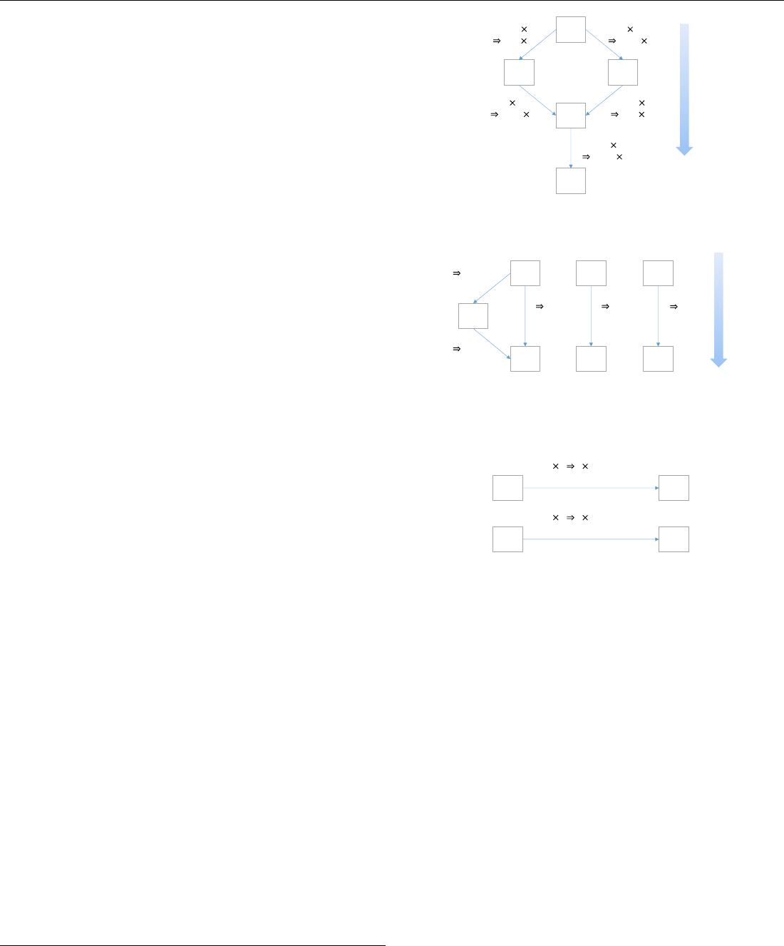
Fig. 1 summarizes the relations among the models A, B, C, D, and E.

Here deep models have smaller ﬁlter sizes. When the time complexity is

roughly the same, the deeper networks with smaller ﬁlters show better re-

sults than the shallower networks with larger ﬁlters.

Trade-offs between Depth and Width

Next we investigate the trade-offs between depth d and width n. We increase

depth while properly reducing the number of ﬁlters per layer, without chang-

ing the ﬁlter sizes. We replace the three 3×3 layers with six 3×3 layers. The

complexity involved is:

128 · 3

· 256 + (256 · 3

· 256) × 2 (2)

= 128 · 3

· 160 + (160 · 3

· 160) × 4 + 160 · 3

· 256.

Here we ﬁx the number of the input channels (128) of the ﬁrst layer, and

the number of output ﬁlters (256) of the last layer, so avoid impacting the

This is an extended abstract. The full paper is available at the Computer Vision Foundation

webpage

ƚŚƌĞĞϯ ϯ

Ɛŝǆ Ϯ Ϯ

ƚǁŽϯ ϯ

ƚŚƌĞĞϯ

ƐŝǆϮ Ϯ

ƚǁŽϯ

ĨŽƵƌϮ Ϯ



ϭϱ͘ϵ



ϭϰ͘ϯ



ϭϰ͘ϵ



ϭϯ͘ϵ



ϭϯ͘ϯ

ĚĞĞƉĞƌΘ

ƐŵĂůůĞƌĨŝůƚĞƌƐ

Figure 1: The relations of the models about depth and ﬁlter sizes.

ĚĞĞƉĞƌΘ

ŶĂƌƌŽǁĞƌ

ϭϰ͘ϴ



ϭϱ͘ϵ

ϭϰ͘ϳ



ϭϰ͘ϯ

ϭϰ͘Ϭ



ϭϯ͘ϵ

ϭϯ͘ϱ

ϯ ϲůĂǇĞƌƐ

;ŽŶƐƚĂŐĞϯͿ

ϴ ůĂǇĞƌƐ

;ŽŶƐƚĂŐĞϯͿ

ϴ ůĂǇĞƌƐ

;ŽŶƐƚĂŐĞϯͿ

Ϯ ϰůĂǇĞƌƐ

;ŽŶƐƚĂŐĞϮͿ

ϰůĂǇĞƌƐ

;ŽŶƐƚĂŐĞϮͿ

Figure 2: The relations of the models about depth and width.

Ϯ Ϯ ϯ ϯ͕ŶĂƌƌŽǁĞƌ

;ŽŶƐƚĂŐĞϯͿ

Ϯ Ϯ ϯ ϯ͕ŶĂƌƌŽǁĞƌ

;ŽŶƐƚĂŐĞϮͿ



ϭϰ͘ϵ

ϭϰ͘ϴ



ϭϯ͘ϯ

ϭϯ͘ϱ

Figure 3: The relations of the models about width and ﬁlter sizes.

previous/next stages. With this replacement, the width reduces from 256 to

160 (except the last layer).

Fig. 2 summarizes the relations among the models of A, F, G, H, and

I. Here the deeper models are narrower. We ﬁnd that increasing the depth

leads to considerable gains, even the width needs to be properly reduced.

Trade-offs between Width and Filter Sizes

We can also ﬁx the depth and investigate the trade-offs between width and

ﬁlter sizes. The models B and F exhibit this trade-off on the last six convo-

lutional layers:

128 · 2

· 256 + (256 · 2

· 256) × 5 (3)

⇒ 128 · 3

· 160 + (160 · 3

· 160) × 4 + 160 · 3

· 256.

This means that the ﬁrst ﬁve 2×2 layers with 256 ﬁlters are replaced with

ﬁve 3×3 layers with 160 ﬁlters.

Fig.

3 shows the relations of these models. Unlike the depth that has a

high priority, the width and ﬁlter sizes (3×3 or 2×2) do not show apparent

priorities to each other.

More trade-offs involving depth, width, ﬁlter sizes, strides, and pooling are

investigated in the main paper.