《TEMPORAL ENSEMBLING FOR SEMI-SUPERVISED LEARNING》 - Samuli Laine.pdf

ghastly

374

13页

0次

2021-08-16

10墨值下载

Published as a conference paper at ICLR 2017

TEMPORAL ENSEMBLING FOR SEMI-SUPERVISED

LEARNING

Samuli Laine

NVIDIA

slaine@nvidia.com

Timo Aila

NVIDIA

taila@nvidia.com

ABSTRACT

In this paper, we present a simple and efﬁcient method for training deep neural

networks in a semi-supervised setting where only a small portion of training data

is labeled. We introduce self-ensembling, where we form a consensus prediction

of the unknown labels using the outputs of the network-in-training on different

epochs, and most importantly, under different regularization and input augmenta-

tion conditions. This ensemble prediction can be expected to be a better predictor

for the unknown labels than the output of the network at the most recent training

epoch, and can thus be used as a target for training. Using our method, we set

new records for two standard semi-supervised learning benchmarks, reducing the

(non-augmented) classiﬁcation error rate from 18.44% to 7.05% in SVHN with

500 labels and from 18.63% to 16.55% in CIFAR-10 with 4000 labels, and further

to 5.12% and 12.16% by enabling the standard augmentations. We additionally

obtain a clear improvement in CIFAR-100 classiﬁcation accuracy by using ran-

dom images from the Tiny Images dataset as unlabeled extra inputs during train-

ing. Finally, we demonstrate good tolerance to incorrect labels.

1 INTRODUCTION

It has long been known that an ensemble of multiple neural networks generally yields better pre-

dictions than a single network in the ensemble. This effect has also been indirectly exploited when

training a single network through dropout (Srivastava et al., 2014), dropconnect (Wan et al., 2013),

or stochastic depth (Huang et al., 2016) regularization methods, and in swapout networks (Singh

et al., 2016), where training always focuses on a particular subset of the network, and thus the com-

plete network can be seen as an implicit ensemble of such trained sub-networks. We extend this idea

by forming ensemble predictions during training, using the outputs of a single network on different

training epochs and under different regularization and input augmentation conditions. Our train-

ing still operates on a single network, but the predictions made on different epochs correspond to an

ensemble prediction of a large number of individual sub-networks because of dropout regularization.

This ensemble prediction can be exploited for semi-supervised learning where only a small portion

of training data is labeled. If we compare the ensemble prediction to the current output of the net-

work being trained, the ensemble prediction is likely to be closer to the correct, unknown labels of

the unlabeled inputs. Therefore the labels inferred this way can be used as training targets for the

unlabeled inputs. Our method relies heavily on dropout regularization and versatile input augmen-

tation. Indeed, without neither, there would be much less reason to place conﬁdence in whatever

labels are inferred for the unlabeled training data.

We describe two ways to implement self-ensembling, Π-model and temporal ensembling. Both ap-

proaches surpass prior state-of-the-art results in semi-supervised learning by a considerable margin.

We furthermore observe that self-ensembling improves the classiﬁcation accuracy in fully labeled

cases as well, and provides tolerance against incorrect labels.

The recently introduced transform/stability loss of Sajjadi et al. (2016b) is based on the same prin-

ciple as our work, and the Π-model can be seen as a special case of it. The Π-model can also be

seen as a simpliﬁcation of the Γ-model of the ladder network by Rasmus et al. (2015), a previously

presented network architecture for semi-supervised learning. Our temporal ensembling method has

connections to the bootstrapping method of Reed et al. (2014) targeted for training with noisy labels.

arXiv:1610.02242v3 [cs.NE] 15 Mar 2017

Published as a conference paper at ICLR 2017

stochastic

augmentation

network

with dropout

cross-

entropy

squared

difference

weighted

sum

loss

stochastic

augmentation

cross-

entropy

squared

difference

weighted

sum

loss

network

with dropout

w(t)

Temporal ensembling

П-model

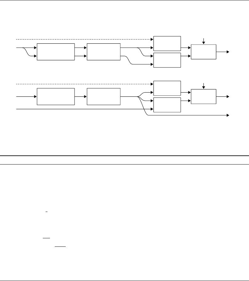
Figure 1: Structure of the training pass in our methods. Top: Π-model. Bottom: temporal en-

sembling. Labels y

are available only for the labeled inputs, and the associated cross-entropy loss

component is evaluated only for those.

Algorithm 1 Π-model pseudocode.

Require: x

= training stimuli

Require: L = set of training input indices with known labels

Require: y

= labels for labeled inputs i ∈ L

Require: w(t) = unsupervised weight ramp-up function

Require: f

(x) = stochastic neural network with trainable parameters θ

Require: g(x) = stochastic input augmentation function

for t in [1, num epochs] do

for each minibatch B do

i∈B

← f

(g(x

i∈B

))  evaluate network outputs for augmented inputs

˜z

i∈B

← f

(g(x

i∈B

))  again, with different dropout and augmentation

loss ← −

|B|

i∈(B∩L)

log z

]  supervised loss component

+ w(t)

C|B|

i∈B

||z

− ˜z

 unsupervised loss component

update θ using, e.g., ADAM  update network parameters

end for

return θ

2 SELF-ENSEMBLING DURING TRAINING

We present two implementations of self-ensembling during training. The ﬁrst one, Π-model, en-

courages consistent network output between two realizations of the same input stimulus, under two

different dropout conditions. The second method, temporal ensembling, simpliﬁes and extends this

by taking into account the network predictions over multiple previous training epochs.

We shall describe our methods in the context of traditional image classiﬁcation networks. Let the

training data consist of total of N inputs, out of which M are labeled. The input stimuli, available

for all training data, are denoted x

, where i ∈ {1 . . . N}. Let set L contain the indices of the labeled

inputs, |L| = M. For every i ∈ L, we have a known correct label y

∈ {1 . . . C}, where C is the

number of different classes.

2.1 Π-MODEL

The structure of Π-model is shown in Figure 1 (top), and the pseudocode in Algorithm 1. During

training, we evaluate the network for each training input x

twice, resulting in prediction vectors z

and ˜z

. Our loss function consists of two components. The ﬁrst component is the standard cross-

entropy loss, evaluated for labeled inputs only. The second component, evaluated for all inputs,

penalizes different predictions for the same training input x

by taking the mean square difference

of 13

10墨值下载

关注

评论