Approximating Median Absolute Deviation With Bounded Error.pdf

Apache IoTDB

179

13页

3次

2023-01-13

免费下载

Approximating Median Absolute Deviation with Bounded Error

Zhiwei Chen, Shaoxu Song

∗

Tsinghua University

{czw18,sxsong}@tsinghua.edu.cn

Ziheng Wei, Jingyun Fang, Jiang Long

Data Governance Innovation Lab, HUAWEI Cloud BU

{ziheng.wei,fangjingyun,longjiang4}@huawei.com

ABSTRACT

The median absolute deviation (MAD) is a statistic measuring the

variability of a set of quantitative elements. It is known to be more

robust to outliers than the standard deviation (SD), and thereby

widely used in outlier detection. Computing the exact MAD how-

ever is costly, e.g., by calling an algorithm of nding median twice,

with space cost

𝑂 (𝑛)

over

𝑛

elements in a set. In this paper, we

propose the rst fully mergeable approximate MAD algorithm, OP-

MAD, with one-pass scan of the data. Remarkably, by calling the

proposed algorithm at most twice, namely TP-MAD, it guarantees

to return an

(𝜖,

)

-accurate MAD, i.e., the error relative to the ex-

act MAD is bounded by the desired

𝜖

or 1. The space complexity

is reduced to

𝑂 (𝑚)

while the time complexity is

𝑂 (𝑛 + 𝑚 log𝑚)

where

𝑚

is the size of the sketch used to compress data, related

to the desired error bound

𝜖

. To get a more accurate MAD, i.e.,

with smaller

𝜖

, the sketch size

𝑚

will be larger, a trade-o between

eectiveness and eciency. In practice, we often have the sketch

size

𝑚 ≪ 𝑛

, leading to constant space cost

𝑂 (

)

and linear time

cost

𝑂 (𝑛)

. The extensive experiments over various datasets demon-

strate the superiority of our solution, e.g., 160000

less memory and

faster than the aforesaid exact method in datasets pareto and

norm. Finally, we further implement and evaluate the parallelizable

TP-MAD in Apache Spark, and the fully mergeable OP-MAD in

Structured Streaming.

PVLDB Reference Format:

Zhiwei Chen, Shaoxu Song and Ziheng Wei, Jingyun Fang, Jiang Long.

Approximating Median Absolute Deviation with Bounded Error. PVLDB,

14(11): 2114-2126, 2021.

doi:10.14778/3476249.3476266

1 INTRODUCTION

Like the standard deviation (SD), the median absolute deviation

(MAD) measures the variability of a quantitative dataset. It is de-

ned as the median of the absolute deviations from the dataset’s

median. For instance, for a dataset

D = {

}

, we

have

MEDIAN =

5. The absolute deviations from the MEDIAN 5

are

{

}

. The MAD of

is thus 2, the MEDIAN of

the absolute deviations.

MAD is practically important for various applications, since it is

a statistic more robust to outliers and long tails than the standard

deviation (SD). For example, Cao et al. [

] use Cauchy distributions

[

] with MEDIAN and MAD of historical query latency data as

∗

Corresponding author

This work is licensed under the Creative Commons BY-NC-ND 4.0 International

License. Visit https://creativecommons.org/licenses/by-nc-nd/4.0/ to view a copy of

this license. For any use beyond those covered by this license, obtain permission by

emailing info@vldb.org. Copyright is held by the owner/author(s). Publication rights

licensed to the VLDB Endowment.

Proceedings of the VLDB Endowment, Vol. 14, No. 11 ISSN 2150-8097.

doi:10.14778/3476249.3476266

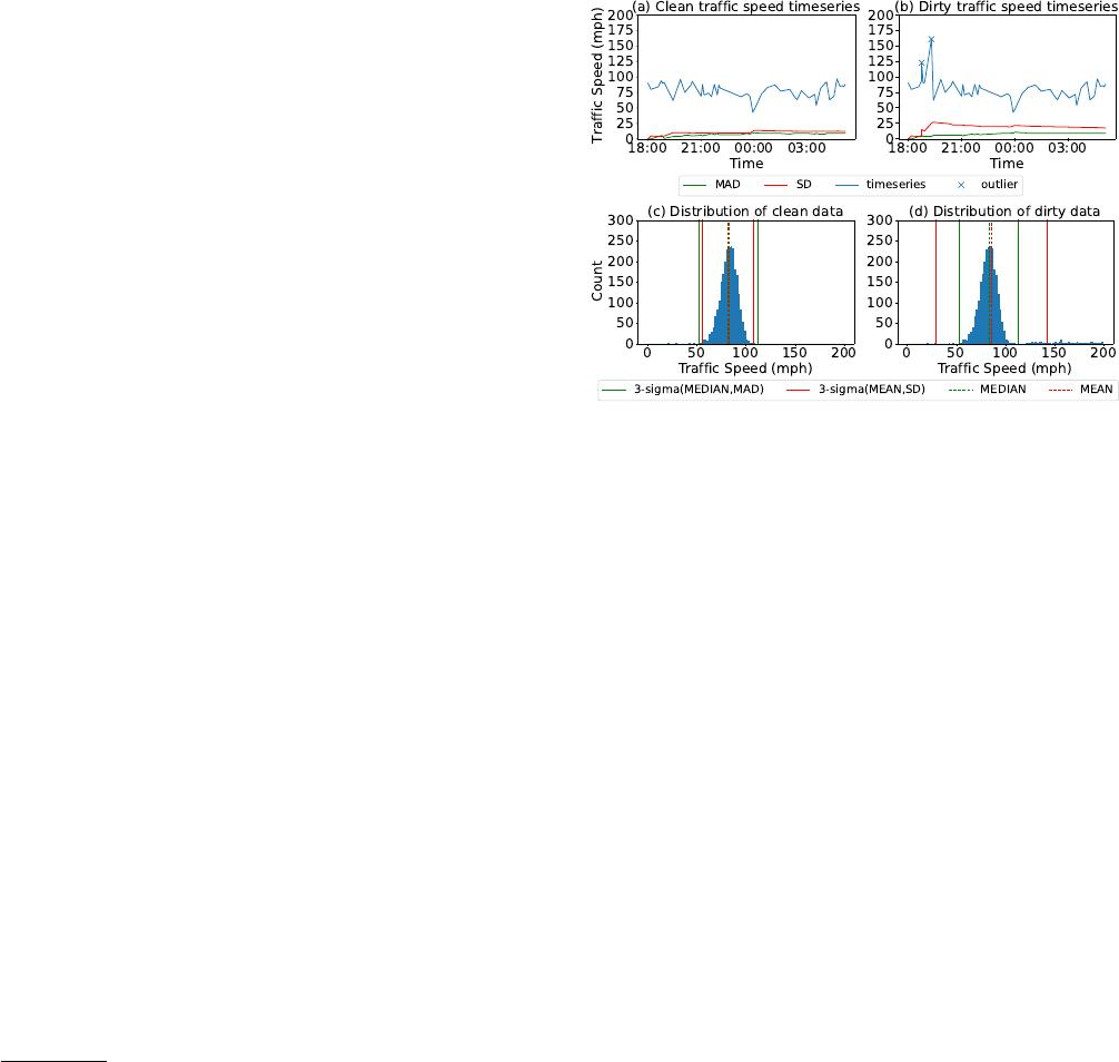
Figure 1: Robustness of median absolute deviation (MAD) to

outliers. The outliers (introduced by errors) in the time se-

ries in (b) signicantly distract the SD statistics, while the

MAD statistics are not aected by such outliers, close to

those in the clean data in (a). When using the 3-sigma rule

for outlier detection, the ranges determined by MEAN and

SD over the dirty data in (d) deviate largely from the truths

in (c), compared to the robust ones by MEDIAN and MAD.

parameters to detect rare or abnormal query events in a database.

They also apply this method to detect anomalous machines, proxy

anomaly and network anomaly. Malinowski et al. [

] use MAD

as a parameter to determine the number of principal factors for

a data matrix in outlier detection. Wu et al. [

] and Adekeye

et al. [

] calculate the limits of control charts with MAD as the

scale parameter for statistical process control. Shawiesh et al. [

]

and Athari et al. [

] use MAD as the estimation of variability to

determine condence intervals for locations of skewed distributions.

Moreover, MAD is applied to image preprocessing, e.g., estimating

noises [

] in gray-scale and colored images using MAD to select

the threshold. As a popular method to preprocess high-throughput

gene expression microarray data, the hit selection method uses

MAD as the parameter of the z score (a hit selection threshold) to

improve the overall selection rates [

]. Software engineers use

MAD as the threshold to classify the defective and clean classes of

datasets from monitoring systems, as an unsupervised method for

software defect prediction [20].

Example 1.1. Figure 1 illustrates the superiority of MAD in out-

lier detection compared to SD. The time series in Figure 1(a) presents

(a segment of) the trac speeds in the Twin Cities Metro area in

Minnesota in NAB [

]. Outliers, e.g., introduced by data errors,

2114

signicantly distract the SD statistics but not MAD, as shown in

Figure 1(b). The K-sigma rule [

] with

𝐾 =

3 detects elements

outside the ranges of solid lines in the distribution as outliers, in

Figure 1(d). Such ranges of solid lines can either be determined

by MEAN and SD (in red), or by MEDIAN and MAD (in green).

As shown in Figure 1(d), the ranges determined by MEDIAN and

MAD are more robust and closer to those over the clean data in

Figure 1(c). The outlier detection by MEDIAN and MAD is thus

more accurate [

]. For instance, the outlier at time 19:00 with value

125, outside the range of green lines, will be detected by MEDIAN

and MAD, but not by MEAN and SD in red lines. ■

Unfortunately, computing the exact MAD over a set of

𝑛

ele-

ments is costly, since it is dened on the median. Unlike SD, which

can be eciently calculated in constant space, the MAD computa-

tion needs to nd the median of the absolute deviations from the

dataset’s median, i.e., nding median twice. Such an exact MAD

algorithm has the space cost

𝑂 (𝑛)

and its time cost depends heavily

on data size, which is not aordable for large scale data. Therefore,

approximate MAD is often considered.

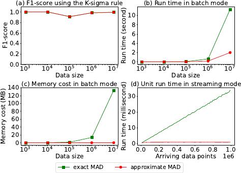
Example 1.2. To demonstrate the suciency and superiority of

approximate MAD compared with exact MAD, we run the outlier

detection application in Example 1.1 over a larger data size with up

to 10

elements. Figure 2 compares the results of approximate MAD

(by Algorithm 2 in Section 3.2) and exact MAD (by Algorithm 3 in

the full version technical report [1]).

(1) Comparable eectiveness. Figure 2(a) with

𝐾 =

7 shows that

the F1-score of outlier detection with approximate MAD is almost

the same as that using exact MAD. That is, it is sucient to use

approximate MAD in this application.

(2) Lower time cost. Figure 2(b) presents the corresponding time

costs of computing approximate MAD and exact MAD in a batch

mode. While their eectiveness of outlier detection is almost the

same as shown in Figure 2(a), the time cost of computing approxi-

mate MAD is only about 1/5 of exact MAD over 10

elements.

(3) Lower space cost. Not only is the time cost saved, as illus-

trated in Figure 2(c), the corresponding space cost of computing

approximate MAD is signicantly lower, almost constant. Given

the almost the same eectiveness but much more ecient time and

space costs, it is sucient to use approximate MAD in practice and

the costly exact MAD is not necessary.

(4) Streaming computation. As presented in Section 3.2, the algo-

rithm for computing approximate MAD can be naturally adapted to

incremental computation for streaming data. In contrast, the exact

MAD needs to scan the entire data, since the set of absolute devia-

tions needs to be reconstructed given a changed median. Therefore,

as illustrated in Figure 2(d), the time cost of computing approximate

MAD is constant in the streaming mode, while that of exact MAD

increases heavily. It demonstrates again the necessity of studying

approximate MAD.

Similarly, the superiority of approximate MAD compared to

exact MAD is also observed in another application of Shewhart

control charts in Figure 11 in Section 5.4. ■

To nd approximate MAD, a natural idea is to nd the approxi-

mate median of the absolute deviations from the dataset’s approxi-

mate median, by calling twice the existing methods of approximat-

ing median [

]. With two median approximations, the error

Figure 2: Superiority of approximate MAD over exact MAD.

(a) Approximate MAD and exact MAD show almost the same

F1-score of outlier detection under various data sizes. The

time costs in (b) and space costs in (c) of computing approxi-

mate MAD are signicantly lower than those of exact MAD,

in a batch mode. (d) The approximate MAD can also be in-

crementally computed in a streaming mode.

introduced by such a simple approximation relative to the exact

MAD is theoretically unknown and practically ineective (see a

detailed discussion in Section 6.1).

To the best of our knowledge, this is the rst study on approxi-

mating MAD with bounded error. Our contributions include

•

an approximate MAD algorithm with explicit error bound,

which is fully mergeable and needs only 1-pass scan of data;

•

a solution by calling the proposed algorithm twice, which is

parallelizable and guarantees to nd an (

𝜖

,1)-accurate MAD;

•

a pruning strategy to skip buckets in the sketch of the second

scan, signicantly reducing the space cost;

•

a distributed implementation in Apache Spark and a stream-

ing implementation in Structured Streaming, both outper-

forming the simple MAD approximation using the built-in

approxQuantile for the approximate median.

Following is the structure of our paper. In Section 2, we rst

give the formal denition of MAD and the measure of approxi-

mate MAD in accuracy. In Section 3, we present the approximate

MAD algorithm and analyze its error bound as well as complex-

ity. In Section 4, we illustrate the solution for approximate MAD

with desired error guarantees, and the bucket pruning strategy.

In Section 5, we compare our solution with several baselines in

experiments, showing the superiority of our proposal in accuracy

and resource occupation. Finally, in Section 6 and Section 7, we

discuss the related work and the conclusion.

Table 1 lists the frequently used notations.

2 FRAMEWORK

In this section, we review the MAD problem together with an exact

computation algorithm, and introduce approximate MAD as well

as the framework of our approximation solution.

2115

of 13

免费下载

文档被以下合辑收录

技术分享（共47篇）

GreatSQL开源数据库是适用于金融级应用的国内自主MySQL版本，专注于提升MGR可靠性及性能，支持InnoDB并行查询等特性，可以作为MySQL或Percona Server的可选替换，用于线上生产环境，且完全免费并兼容MySQL或Percona Server。

关注

文档被以下合辑收录

评论