


先说个好消息, Qwen2 来了,并且可以通过ollama下载了
前言
在研究全文索引的时候,找到一篇不错的文章,Building an efficient sparse keyword index in Python[1], 它比较了三种全文索引方法,
• rank,即之前文章提到的
rank_bm25
的BM25Okapi• sqlite, 利用SQLite的 FTS5
• scoring txtai[2] 实现的BM25,
💡:txtai 使用了pickle(score) 和sqlite3(terms)的混合方案,所以我个人还是推荐SQLite FTS5的方案,依赖更少,并且有中文索引插件(下期讨论) 如果想要下载本文代码和数据集,可以私信bm25。
正文
语义搜索是一种基于自然语言处理(NLP)最新进展的新型搜索类别。传统的搜索引擎使用关键词来查找数据。语义搜索具有对自然语言的理解,并识别具有相同含义的结果,而不仅仅是相同的关键词。
虽然语义搜索增加了惊人的功能,但稀疏关键词索引仍然可以增加价值。可能存在需要找到精确匹配的情况,或者我们只是想要一个快速的索引来迅速扫描数据集。
不幸的是,基于 Python 的关键词索引库并没有太多优秀的选择。可用的选项大多无法扩展或效率极低,仅适用于简单情况。
由于 Python 是一种解释型语言,从性能角度来看,它经常受到负面评价。在某些情况下,这种评价是有道理的,因为 Python 可能会消耗大量内存,并且具有全局解释器锁(GIL),这会强制单线程执行。但确实有可能构建与其它语言性能相当的高效 Python 代码。
本文将探讨如何在 Python 中构建高效的稀疏关键词索引,并与其他方法进行比较。
安装依赖项
安装 txtai
及其所有依赖项。
# Install txtai
pip install txtai pytrec_eval rank-bm25 elasticsearch==7.10.1
引入问题
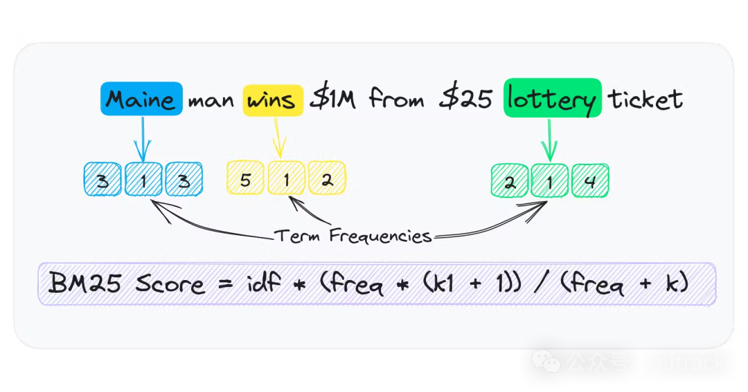
关键词索引通过将文本分词为每篇文档的令牌列表来工作。这些令牌按文档汇总频率,并存储在术语频率稀疏数组中。
词频数组在只存储词条存在于文档中的频率时是稀疏的。例如,如果一个词条存在于 1000 份文档中的 1 份中,稀疏数组只有一个条目。稠密数组存储了 1000 个条目,除了一个之外都为零。
存储一个词频稀疏数组的简单方法之一是为每个单词拥有一个字典 {id: frequency}
。这种方法的问题在于 Python 具有显著的对象开销。
让我们检查单个数字所使用的大小。
import sys

a = 100
sys.getsizeof(a)
# 28
单个整数需要 28 字节。与本地的 int/long(分别为 4 或 8 字节)相比,这相当浪费。想象一下有成千上万的 id: frequency
映射。内存使用量将迅速增长。
让我们演示一下。下面的代码运行一个包含 Python 进程,该进程生成一个包含一千万个数字的列表。
运行作为单独的进程有助于计算更准确的内存使用统计信息。
import psutil

results = []
for x in range(int(1e7)):
  results.append(x)

print(f"MEMORY USAGE = {psutil.Process().memory_info().rss / (1024 * 1024)} MB")
MEMORY USAGE = 394.640625 MB
这段数组使用了大约 395MB(我的电脑返回374.53125MB
) 的内存。这似乎有些高。
Python的高效数值数组
幸运的是,Python 有一个用于构建高效数值数组[3]的模块。该模块允许构建具有相同原生类型的数组。
让我们尝试使用一种 long long
类型,它占用 8 字节。
from array import array

import psutil

results = array("q")
for x in range(int(1e7)):
  results.append(x)

print(f"MEMORY USAGE = {psutil.Process().memory_info().rss / (1024 * 1024)} MB")
MEMORY USAGE = 88.54296875 MB
如我们所见,内存使用从 395MB 减少到 89MB。这是 4 倍的减少,与之前的计算结果每数字 28 字节相比每数字 8 字节是一致的。
高效处理数值数据
纯 Python 的大计算也会非常缓慢。幸运的是,数值处理有丰富的选项。最流行的框架是 NumPy[4].。还有 PyTorch[5] 和其他基于 GPU 的张量处理框架。
以下是用于演示 Python 与 NumPy 对数组进行排序的简单示例。
import random
import time

data = [random.randint(1, 500) for x in range(1000000)]

start = time.time()
sorted(data, reverse=True)
print(time.time() - start)
# 0.08496785163879395
import numpy as np

data = np.array(data)

start = time.time()
np.sort(data)[::-1]
print(time.time() - start)
# 0.030919790267944336
如我们所见,NumPy 中对数组进行排序要快得多。这可能看起来不多,但在大量运行时这一点会累积起来。
txtai 中的稀疏关键词索引
既然我们已经讨论了关键性能概念,接下来让我们谈谈如何将这些应用到构建稀疏关键词索引中。
返回原始方法处理词频稀疏数组,我们发现使用 Python 的 array 包更为高效。在 txtai 中,这种方法用于为每个词构建词频数组。这导致了接近原生的速度和内存使用。
搜索方法利用了多个 NumPy 方法高效计算查询词匹配。每个查询都会被分词,并获取那些词频数组来计算查询得分。这些 NumPy 方法都是用 C 语言编写的,通常会释放 GIL。因此,再次实现了接近原生的速度和能够使用多线程的能力。
在 GitHub 上阅读完整的实现[6],以了解更多信息。
评估性能
首先,回顾一下当前的搜索环境。正如在介绍中提到的那样,并没有太多优秀的选择。Apache Lucene[7] 无疑是从速度、性能和功能角度来看最好的传统搜索索引, 它是 Elasticsearch/OpenSearch 和其他许多项目的基础。但它需要 Java 的支持。
算法
• Rank-BM25[8]
• SQLite FTS5[9]
• txtai BM25[10]
数据集
我们将使用 BEIR 数据集。我们还将使用来自 txtai 项目的基准脚本。这个基准脚本具有与 BEIR 数据集交互的方法。
性能测试脚本中需要注意以下几点重要提示。
• 对于 SQLite FTS 实现,每个词元通过
OR
子句连接在一起。默认情况下,SQLite FTS 会通过AND
子句隐式地将子句连接在一起。相比之下,Lucene 的默认操作符是OR
。• Elasticsearch 实现使用 7.x,因为它在笔记本中实例化更简单。
• 除了 Elasticsearch 之外的所有方法都使用 txtai 的 Unicode 分词器(unicode tokenizer[11])对文本进行分词以保持一致性
下载benchmarks.py和数据集
import os

# Get benchmarks script
os.system("wget https://raw.githubusercontent.com/neuml/txtai/master/examples/benchmarks.py")

# Create output directory
os.makedirs("beir", exist_ok=True)

# Download subset of BEIR datasets
datasets = ["trec-covid", "nfcorpus", "webis-touche2020", "scidocs", "scifact"]
for dataset in datasets:
  url = f"https://public.ukp.informatik.tu-darmstadt.de/thakur/BEIR/datasets/{dataset}.zip"
  os.system(f"wget {url}")
  os.system(f"mv {dataset}.zip beir")
  os.system(f"unzip -d beir beir/{dataset}.zip")

  # Remove existing benchmark data
if os.path.exists("benchmarks.json"):
  os.remove("benchmarks.json")
基准测试
从这里开始,和原文不一样,因为benchmarks.py
更新了
datasets = ["trec-covid", "nfcorpus", "webis-touche2020", "scidocs", "scifact"]
# Runs benchmark evaluation
def evaluate(method):
  for dataset in datasets:
    command = f"python benchmarks.py -d beir -s {dataset} -m {method} -r"
    print(command)
    os.system(command)

# Calculate benchmarks
for method in [ "rank", "sqlite","scoring"]:
  evaluate(method)
读取测试结果,生成测试报告
import json
import pandas as pd

def benchmarks():
  df = pd.read_json("benchmarks.json", lines=True).sort_values(by=["source", "search"])
  return df[["source", "method", "index", "memory", "search", "ndcg_cut_10", "map_cut_10", "recall_10", "P_10"]].reset_index(drop=True)

# Load benchmarks dataframe
df = benchmarks()
df.groupby(['source','method']).max().reset_index()
| source | method | index | memory | search | ndcg_cut_10 | map_cut_10 | recall_10 | P_10 | |
| 0 | nfcorpus | rank | 0.59 | 609 | 4.34 | 0.30692 | 0.11711 | 0.1532 | 0.21889 |
| 1 | nfcorpus | scoring | 0.94 | 574 | 0.29 | 0.30639 | 0.11728 | 0.14891 | 0.21734 |
| 2 | nfcorpus | sqlite | 0.51 | 544 | 2.73 | 0.30695 | 0.11785 | 0.14871 | 0.21641 |
| 3 | scidocs | rank | 3.55 | 949 | 45.91 | 0.14932 | 0.0867 | 0.15408 | 0.0761 |
| 4 | scidocs | scoring | 5.17 | 668 | 0.39 | 0.15063 | 0.08756 | 0.15637 | 0.0772 |
| 5 | scidocs | sqlite | 3.36 | 595 | 17.54 | 0.15156 | 0.08822 | 0.15717 | 0.0776 |
| 6 | scifact | rank | 0.79 | 632 | 8.01 | 0.65618 | 0.61204 | 0.774 | 0.085 |
| 7 | scifact | scoring | 1.18 | 579 | 0.3 | 0.66324 | 0.61764 | 0.78761 | 0.087 |
| 8 | scifact | sqlite | 0.69 | 554 | 6.14 | 0.6663 | 0.61966 | 0.79494 | 0.088 |
| 9 | trec-covid | rank | 20.06 | 3035 | 21.33 | 0.57773 | 0.0121 | 0.0155 | 0.632 |
| 10 | trec-covid | scoring | 27.52 | 1152 | 0.12 | 0.58119 | 0.01247 | 0.01545 | 0.618 |
| 11 | trec-covid | sqlite | 19.44 | 817 | 8.67 | 0.56778 | 0.0119 | 0.01519 | 0.61 |
| 12 | webis-touche2020 | rank | 73.89 | 8248 | 29.43 | 0.39861 | 0.16492 | 0.2377 | 0.36122 |
| 13 | webis-touche2020 | scoring | 98.52 | 1515 | 0.17 | 0.3692 | 0.14588 | 0.22736 | 0.34694 |
| 14 | webis-touche2020 | sqlite | 68.63 | 1369 | 12.01 | 0.37194 | 0.14812 | 0.2289 | 0.35102 |
上文显示了每个来源和方法的指标。
表格标题列出了 source (dataset)
、 index method
、 index time(s)
、 memory usage(MB)
、 search time(s)
和 NDCG@10
/ MAP@10
/ RECALL@10
/ P@10
的准确性指标。
如我们所见,txtai 的实现具有最快的搜索时间。但在索引时间方面较慢。准确性指标略有差异,但每种方法下的值大致相同。
内存使用量突出。SQLite 和 txtai 在每个源的使用量大致相同。Rank-BM25 的内存使用量可能会迅速失控。例如, webis-touch2020
,仅包含约 40 万条记录,使用的内存为 8 GB
,而其他实现方式则为 1.5GB
左右 。
与 Elasticsearch 比较
💡:从这里开始,我没有做测试,有兴趣的,自行测试比较 既然我们已经回顾了在 Python 中构建关键词索引的方法,现在让我们看看 txtai 的稀疏关键词索引与 Elasticsearch 相比如何。
我们将启动一个内置实例并运行相同的评估。
# Download and extract elasticsearch
os.system("wget https://artifacts.elastic.co/downloads/elasticsearch/elasticsearch-7.10.1-linux-x86_64.tar.gz")
os.system("tar -xzf elasticsearch-7.10.1-linux-x86_64.tar.gz")
os.system("chown -R daemon:daemon elasticsearch-7.10.1")
from subprocess import Popen, PIPE, STDOUT

# Start and wait for server
server = Popen(['elasticsearch-7.10.1/bin/elasticsearch'], stdout=PIPE, stderr=STDOUT, preexec_fn=lambda: os.setuid(1))
# Add benchmark evaluations for Elasticsearch
evaluate("es")

# Reload benchmarks dataframe
df = benchmarks()
再次,txtai 的实现与 Elasticsearch 相比表现良好。准确性指标有所不同,但大致相同。
重要的是要注意,在使用固态存储进行内部测试时,Elasticsearch 和 txtai 的速度大致相同。在 Google Colab 环境下运行时,Elasticsearch 速度略慢的情况是其产品特性。
收尾
这本笔记本展示了如何在 Python 中构建高效的稀疏关键词索引。基准测试表明,txtai 提供了强大的实现,无论从准确性和速度方面来看,都与 Apache Lucene 相当。
这个关键词索引可以作为 Python 中的独立索引使用,也可以与稠密向量索引结合形成一个 hybrid
索引。
RAG开发系列
引用链接
[1]
Building an efficient sparse keyword index in Python: https://neuml.hashnode.dev/building-an-efficient-sparse-keyword-index-in-python[2]
txtai: https://github.com/neuml/txtai[3]
数组: https://docs.python.org/3/library/array.html[4]
NumPy: https://github.com/numpy/numpy[5]
PyTorch: https://github.com/pytorch/pytorch[6]
GitHub 上阅读完整的实现: https://github.com/neuml/txtai/blob/master/src/python/txtai/scoring/terms.py[7]
Apache Lucene: https://github.com/apache/lucene[8]
Rank-BM25: https://github.com/dorianbrown/rank_bm25[9]
SQLite FTS5: https://www.sqlite.org/fts5.html[10]
txtai BM25: https://github.com/neuml/txtai/blob/f28225b0916e886cce313f067c0cd75a6541d6bf/src/python/txtai/scoring/bm25.py[11]
unicode tokenizer: https://github.com/neuml/txtai/blob/master/src/python/txtai/pipeline/data/tokenizer.py
